Networking for Nutanix Flow: The Prerequisites

September 9, 2026

Fundamentals · Prerequisites · Nutanix Flow

The general networking you need in order to read a Flow Virtual Networking and Flow Network Security study guide without stopping every third paragraph. Vendor neutral fundamentals, with a note at the end of each section on where Flow uses them.

Most people who end up owning Nutanix Flow did not come from a networking background. They came from virtualization, or storage, or the platform team, and Flow arrived as a checkbox in Prism Central that suddenly required them to have opinions about BGP session states and MTU arithmetic. The Nutanix documentation is good at telling you which field to fill in. It is not written to teach you why the field exists.

This is the missing layer underneath. It is not a networking course and it is not exam material. It is the set of concepts that a Flow study guide assumes you already have, arranged in the order you will hit them, with the Flow specific payoff called out so you can see why each one matters.

What this is. Standards based networking fundamentals, independent of any vendor. Where a concept has a Nutanix specific twist, that appears in a marked Where Flow uses this block so you can tell the general from the product specific.

What this is not. Nutanix documentation, exam content, or a substitute for either. Nothing here is sourced from a Nutanix guide, because none of it is Nutanix specific. Protocol references are given for orientation; verify them at the source before quoting them anywhere that matters.

1. Layer 2: frames, MAC addresses, and VLANs

A switch moves frames. A frame carries a source and destination MAC address, which is a 48 bit hardware identifier burned into a NIC, or assigned to a virtual NIC by the hypervisor.

Switches are not configured with a map of where things are. They learn. When a frame arrives on a port, the switch records “source MAC X lives on port 3” in its MAC address table. When a frame needs to go to a destination it has already learned, it sends it out that one port. This is why switching scales.

The three things a switch does with a frame

Case	Behaviour	Name
Destination MAC is in the table	Send out that single port	Forwarding
Destination MAC is not in the table	Send out every port except the one it arrived on	Unknown unicast flooding
Destination is the broadcast address `ff:ff:ff:ff:ff:ff`	Send out every port except the one it arrived on	Broadcast

Unknown unicast flooding is the one worth remembering, because it is a behaviour some applications quietly depend on, and modern virtual networking often disables it. Clustered applications that expect to receive traffic for a MAC they have not yet announced will break when flooding is turned off, and the failure looks like an application problem rather than a network one.

Broadcast domains and why VLANs exist

Every port that can receive a given broadcast is in the same broadcast domain. One flat switched network is one broadcast domain, and every device in it hears every broadcast. That does not scale, and it provides no separation at all.

A VLAN cuts one physical switch into several logical switches. Ports in VLAN 10 cannot see traffic in VLAN 20 without something routing between them. VLAN IDs run from 1 to 4094, which is both the strength and the ceiling of the technology.

Two port types, one common source of confusion. Most VM facing ports are access ports. Host uplinks are usually trunks.

Access port. Belongs to exactly one VLAN. The endpoint sends and receives ordinary untagged frames and has no idea VLANs exist. This is how most VMs are connected.
Trunk port. Carries several VLANs, tagging each frame with a 4 byte 802.1Q header so the far end can separate them. This is how a hypervisor host uplink normally connects to the physical switch.
Native or untagged VLAN. The one VLAN on a trunk whose frames travel with no tag. Mismatched native VLANs on the two ends of a trunk is a classic and very confusing outage.

ARP, the glue between Layer 2 and Layer 3

A host that wants to send to an IP address on its own subnet does not know the destination MAC. It broadcasts an ARP request: “who has 10.0.0.5?” The owner replies with its MAC, the sender caches it, and the conversation proceeds.

Two consequences worth carrying:

ARP is a broadcast, so it is confined to the broadcast domain. This is why a VLAN boundary is a real boundary.
ARP caches go stale. When something moves, or something else starts answering for an address, traffic follows the cache and not reality until the entry ages out. A surprising number of “the network is broken” incidents are stale or contested ARP.

Where Flow uses this

Flow subnets come in two shapes, VLAN backed and overlay backed, and the guide distinguishes them constantly. Flow also disables unknown unicast flooding on its own VLAN subnets, which is called out as a limitation rather than a feature, and it is the reason some workloads cannot be migrated onto them. When a subnet is stretched between sites, ARP behaviour becomes the central problem rather than a detail: something has to answer ARP for an address that lives somewhere else.

2. Layer 3: addresses, prefixes, and routes

Routing moves packets between subnets. Where switching asks “which port has this MAC”, routing asks “which next hop gets me closer to this network”.

Reading CIDR without thinking about it

An address like 10.20.30.0/24 is a network address and a prefix length. The prefix length says how many leading bits are the network portion. Everything after is host space.

Prefix	Mask	Usable hosts	Typical use
/24	255.255.255.0	254	The standard VM subnet
/25	255.255.255.128	126	Half a /24
/30	255.255.255.252	2	Classic router to router link
/31	255.255.255.254	2	Modern point to point link
/32	255.255.255.255	1	A single host route
/16	255.255.0.0	65,534	A large block, often subdivided
/0	0.0.0.0	everything	The default route

Smaller number means bigger network. A /16 contains 256 /24s. That inversion is the single most common stumbling block for people new to this.

Private address space

Three ranges are reserved for internal use and are never routed on the public internet, defined in RFC 1918:

10.0.0.0/8, a very large flat block
172.16.0.0/12, which is 172.16 through 172.31 and catches people out
192.168.0.0/16

Because everyone uses the same private ranges, overlapping address space between two organizations, or between two tenants, is normal rather than exceptional. Every technology in this document that involves joining two networks has to have an answer for it.

The routing table and longest prefix match

A routing table is a list of destinations and next hops. When a packet arrives, the router checks every entry that could contain the destination and picks the one with the longest prefix, meaning the most specific match. It does not pick the first match, or the cheapest, until specificity has already tied.

Specificity wins before anything else does. A default route only ever gets used when nothing more specific matches.

The default route, 0.0.0.0/0, matches everything and is therefore always the least specific entry in the table. It is the catch all for “I do not have a better idea, send it to the edge”. Any network that needs to reach things outside itself needs one, or an explicit route for every destination it cares about.

The next hop is the address of the neighbouring router that will take the packet onward. It is always an address the router can already reach directly, which is why a next hop outside the local subnet is a configuration error rather than a clever shortcut.

Static versus dynamic routing

Static routes are typed in by a human. They are predictable, they never converge on a new path, and they are silently wrong the moment the topology changes.
Dynamic routing protocols let routers tell each other what they can reach, and recompute when something fails. In this world that means BGP, with OSPF appearing occasionally inside a single site.

Where Flow uses this

A Flow VPC has its own routing table, and the guide talks constantly about the default route pointing at an external subnet as the next hop, about destination prefixes deciding which external subnet a given destination uses, and about selection between them being by longest prefix match. Externally Routable Prefixes are just a list of prefixes the VPC is willing to advertise. None of that is unusual routing, it is ordinary routing expressed in Nutanix nouns.

3. BGP, only the parts Flow uses

BGP is the routing protocol of the internet and, increasingly, of the data centre. It is large. Flow uses a small and well defined corner of it, and you can read the entire Flow BGP surface knowing six things.

One: autonomous systems and the two flavours of BGP

An autonomous system is a network under one administrative control, identified by an ASN. Private ASNs exist for internal use, the same way private IP ranges do.

eBGP runs between different autonomous systems. Different ASN on each end.
iBGP runs inside one autonomous system. Same ASN on both ends.

They behave differently in ways that matter to a network engineer and barely at all here. What matters is that when a product says “eBGP”, it is telling you the two ends are meant to be separately administered networks that agree to exchange routes.

Two: a session is a TCP connection, and its state has a trap in it

BGP peers establish a TCP connection, on port 179, and exchange routes over it. The session walks through a state machine. Only one state means the session is working.

State	Meaning	Good?
Idle	Not attempting. Usually administratively down or backing off after failures	No
Connect	Waiting for the TCP connection to complete	In progress
Active	Actively trying to establish and failing. The name is a trap	No
OpenSent / OpenConfirm	Negotiating parameters	In progress
Established	The session is up and routes are being exchanged	Yes

The single most useful thing in this section In BGP, “Active” does not mean healthy. It means trying and not succeeding. A session sitting in Active is a broken session, and it usually points at the peer, the underlay path, or an ASN or address mismatch, rather than at anything in your own session configuration. Every monitoring screen that shows you “Established or Active” is showing you “up or down” in protocol vocabulary.

Three: advertisement is a choice, not a consequence

A BGP speaker does not automatically tell its neighbour about everything it knows. It advertises what its policy says to advertise. If a prefix is not reaching a peer, the first question is not “is the session up” but “is this prefix in what we advertise to that peer”.

Four: path selection, and the two ways to influence it

When the same destination is learned from more than one peer, BGP picks one path using a long ordered list of tie breakers. Two of them are the ones you will actually see exposed in products.

Lever	Direction	What it does
Local preference, or any vendor’s “route priority” knob	Inbound, affects your own choices	Tells your routers which learned path to prefer. Higher wins. Never leaves your AS
AS Path prepending	Outbound, affects the neighbour’s choices	Repeats your own ASN in the path so the route looks longer and therefore worse. This is how you make a path less preferred as seen by someone else

The asymmetry is the point. You control your own preferences directly. You can only influence someone else’s, and the polite way to do it is to make your own route look worse, not to try to make it look better.

Prepending is a lever on someone else’s decision, applied by degrading your own advertisement.

Five: communities are tags, and that is all

A BGP community is a label attached to a route, conventionally written ASN:value. BGP itself does nothing with them. They exist so that routers downstream can match on the tag and apply policy. Think of them as sticky notes that survive the journey.

Six: what a healthy BGP relationship needs

IP reachability between the two peer addresses before BGP can do anything. BGP rides on TCP and TCP needs a working path.
Matching expectations about ASN and peer address on both ends.
Optionally an MD5 password on the session. Worth knowing because address translation between the peers breaks password verification, since the authentication covers header fields that NAT rewrites.

Where Flow uses this

Flow exposes exactly this subset: eBGP sessions to physical routers, an ASN on each side, a route priority number, AS Path prepending, community tags, and a choice of which Externally Routable Prefixes to advertise. The status fields it shows you are the protocol states above. It does not expose BFD, timer tuning or graceful restart, so if you go looking for them you will not find them. And the MD5 password caveat is why the documentation says passwords cannot be used where the gateway sits behind NAT.

4. NAT, SNAT, and floating IPs

Network Address Translation rewrites addresses in a packet as it crosses a boundary. It exists because private address space is not routable outside, and because organizations run out of public addresses.

Kind	What it rewrites	Direction it enables	Typical use
SNAT, source NAT	The source address of outbound packets, usually to one shared address, tracking sessions by port	Outbound only. Many private hosts share one public address	Giving a whole subnet internet access
DNAT, destination NAT	The destination address of inbound packets	Inbound. Publishes an internal service on an external address	Port forwarding, publishing a web server
Static or 1:1 NAT	Both directions, one external address bound to one internal address	Both. The host is reachable in and out	A server that must both initiate and receive

The asymmetry is the thing to internalise. SNAT alone gives you outbound connectivity and no inbound reachability, because there is nothing to tell the translator which internal host an unsolicited inbound packet was meant for. That is not a bug, it is often the point.

A floating IP is the cloud name for static 1:1 NAT with an address that can be detached from one workload and attached to another.

Floating IPs

A floating IP is an externally routable address held by the platform rather than by a machine, and bound to a workload on request. It is 1:1 NAT with a management story: the address survives the workload, so you can move it to a replacement instance without anything downstream needing to change.

What NAT quietly breaks

Anything that authenticates the header. BGP MD5 and IPsec AH both cover fields NAT rewrites.
Anything that carries an address inside the payload. The classic examples are FTP and SIP, which announce addresses in the data stream that the translator does not know to rewrite.
End to end identity in logs. Behind SNAT, everything appears to come from one address, which matters more than people expect when investigating an incident.

Where Flow uses this

A Flow VPC attaches to the outside through an external subnet that is either NAT or No-NAT. NAT gives the VPC a SNAT address for outbound and floating IPs for selective inbound. No-NAT skips translation entirely and advertises the internal prefixes to the physical network over BGP, which is why No-NAT and Externally Routable Prefixes always appear together. The choice between them is the choice between “hide behind one address” and “make these prefixes genuinely routable”.

5. Overlay and underlay

This is the concept that makes modern virtual networking make sense, and it is one idea: put a whole network inside packets on another network.

The underlay is the real physical network. Switches, cables, IP addresses, ordinary routing. It has one job: carry packets between hosts.
The overlay is a virtual network built on top, whose packets are wrapped inside underlay packets and carried across as ordinary payload.

The underlay does not know the overlay exists. It sees normal UDP traffic between two host addresses. All the tenant structure, the VLANs, the addressing, lives in the wrapper.

Every overlay technology looks like this. Only the size and shape of the wrapper differs.

The encapsulation formats you will meet

Format	Header shape	Notes
VXLAN	Outer Ethernet, outer IP, UDP, then a fixed 8 byte VXLAN header	The older and simpler of the two. Widely supported in hardware. Carries a 24 bit segment ID, so roughly 16 million segments against a VLAN’s 4094
Geneve	The same outer headers, then an 8 byte base header plus variable length options	Designed to be extensible, which is why its overhead is larger and not a single fixed number

Where the byte counts come from, and a caution The outer wrapper for both formats is 14 bytes of Ethernet, 20 bytes of IPv4 and 8 bytes of UDP, which is 42 bytes. VXLAN adds a fixed 8, giving the 50 bytes you will see quoted everywhere. Geneve adds an 8 byte base header plus whatever options the implementation uses, so Geneve overhead is a range, not a constant, and a vendor quoting a single Geneve number is quoting their own implementation.

That arithmetic is mine, not a citation. It is standard and easy to verify, but if a specific byte count matters to a design, take it from the platform’s own documentation rather than from a general calculation.

VTEP: where the wrapping happens

A VTEP, tunnel endpoint, is the thing that adds the wrapper on the way in and strips it on the way out. It can be a physical switch, or software inside a hypervisor. Two VTEPs with underlay reachability between them can carry an overlay segment between them, and the underlay never needs to be told.

This is the whole trick, and it explains why overlays are attractive: the tenant topology becomes software, and the physical network stops needing to change every time the tenant topology does.

Where Flow uses this

Flow overlay subnets are Geneve encapsulated between AHV hosts. Flow also uses VXLAN, separately, when extending a Layer 2 segment to another site or to a non Nutanix device, and it calls those endpoints VTEP gateways. So both formats appear, doing different jobs: Geneve for intra cluster overlay, VXLAN for inter site extension. When both are in play the overheads stack, which is the subject of the next section.

6. MTU, which is where most of this actually goes wrong

If you learn one thing here, learn this one. Encapsulation problems almost always present as MTU problems, and MTU problems present as some of the most misleading symptoms in networking.

The two numbers

MTU, maximum transmission unit, is the largest payload a link will carry in one frame. The classic Ethernet value is 1500 bytes.
MSS, maximum segment size, is the largest chunk of TCP data in one segment. For IPv4 it is conventionally MTU minus 40, being 20 bytes of IP header and 20 of TCP header.

Jumbo frames

A jumbo frame is anything above the standard 1500, and 9000 is the near universal convention. It exists to reduce per packet overhead on high throughput links, and in the overlay world it exists to give you headroom to absorb encapsulation without shrinking the guest.

Jumbo frames only work end to end Every device in the path has to agree. One switch port left at 1500 in an otherwise 9000 path does not degrade gracefully. Small packets succeed and large packets vanish, which means ping works, SSH works, logins work, and then a file copy or a database query hangs. People spend days on this. When you configure jumbo frames on the physical switches, configure a little headroom above 9000 so the switch can carry the frame plus its own tags.

The arithmetic of stacked overhead

If the underlay stays at 1500 and the guest keeps its own MTU at 1500, the encapsulated frame does not fit. Something must give. Either the underlay grows, or the guest shrinks by exactly the overhead:

What is in the path	Overhead	Guest MTU if the underlay stays at 1500
Overlay only, Geneve	58	1442
Overlay plus Layer 2 extension over VXLAN	58 + 50	1392
Overlay plus IPsec VPN	58 + 86	1356
Overlay plus VXLAN plus IPsec	58 + 50 + 86	1306

Overheads stack. Each tunnel you nest costs its own headers. This is why the guidance for a simple overlay and the guidance for an extended, encrypted overlay are not the same number, and why a fallback value that works for the simple case is not enough for the complex one.

Path MTU Discovery, and how it gets broken

A sender does not know the smallest MTU along the path. Path MTU Discovery finds it: the sender marks packets Do Not Fragment, and any router that cannot forward one replies with an ICMP Destination Unreachable, Fragmentation Needed message, type 3 code 4, carrying the MTU it can accept. The sender shrinks and retries.

The ICMP black hole If something in the path blocks ICMP, that reply never arrives. The sender keeps sending packets that are too large, gets no error, and simply sees them disappear. The connection establishes, small exchanges work, and bulk transfer hangs forever.

This is why “we block ICMP for security” is one of the most expensive habits in enterprise networking, and why a security policy that drops ICMP can break things that look nothing like ICMP. It is also why several health check mechanisms treat an ICMP unreachable as meaningful signal rather than noise.

Where Flow uses this

This is the source of the apparent contradiction that trips up most Flow readers: the Controller VM MTU must stay at 1500, yet Flow wants jumbo frames. Both are true and they are about different interfaces. The CVM’s own traffic is never encapsulated, so it has no overhead to absorb. The jumbo frame recommendation applies to the physical switches, the host uplinks and the virtual switch, which is where the Geneve wrapper is actually paid for. Raising the underlay lets guests keep a 1500 byte MTU; leaving it at 1500 means every guest in a VPC has to come down to 1442. The documented fallback is exactly that, and it is a real option, just an operationally annoying one.

7. The hypervisor is a switch

Inside every virtualization host there is a software switch. VM virtual NICs plug into it, and it plugs into the physical NICs. Understanding its parts removes most of the mystery from host networking.

Term	What it is
Bridge	The software switch itself, on one host. Open vSwitch calls the default one `br0`
Virtual switch	A management abstraction over the same bridge on every host in the cluster, so you configure once instead of per host. The default is usually named `vs0`
Uplink	A physical NIC attached to the bridge, connecting it to the outside world
Bond, or NIC team	Several uplinks grouped together for redundancy, throughput, or both

Bond modes, and why the choice matters

Mode	How traffic is placed	Needs switch configuration?
Active backup	One uplink carries everything. The others wait	No. Simplest and most forgiving. No aggregate throughput gain
Balance SLB, source load balancing	Spreads by source MAC across uplinks	No. Gives some spread without switch involvement
Balance TCP, with LACP	Hashes each flow across all uplinks	Yes. The physical switch must run LACP on a matching port channel

LACP, standardised as 802.3ad, is the protocol two ends use to agree that a set of links is one logical link. It has a negotiation rate, fast or slow, and both ends should agree. It also has a failure behaviour worth knowing: if negotiation does not complete, you want the switch to fall back to treating the ports as individual links rather than leaving them all down, otherwise a partial misconfiguration takes the host completely offline.

Consistency is a hard requirement, not a preference Bond modes and bridge names have to be identical on every host in a cluster. A cluster where some hosts run active backup and others run balance TCP will pass every test you run on a quiet day and then fail during a rolling upgrade, when a VM migrates onto a host whose networking behaves differently. Most platform level “virtual switch migration failed” errors trace back to exactly this.

Where Flow uses this

Flow inherits all of it. Virtual switch vs0 and bridge br0 are the defaults everywhere in the documentation, and Flow adds its own bridge for overlay traffic alongside them. Segregating overlay traffic onto a second virtual switch is the standard method for keeping tenant traffic off the management VLAN. The requirements about identical bond types across hosts, LACP fast rate, and spanning tree portfast on the switch ports are not Flow inventions; they are ordinary host networking requirements that Flow surfaces because Flow operations trigger rolling restarts that expose them.

8. Stateful firewalling and microsegmentation

The five tuple

A network conversation is identified by five values. Nearly every firewall, load balancer and flow record in existence is built on them:

Field	Example
Source IP	10.20.30.40
Destination IP	10.50.60.70
Source port	51234, usually ephemeral
Destination port	443
Protocol	TCP

Stateless versus stateful

A stateless filter evaluates each packet on its own. It has no memory. To allow a conversation you must write a rule for the request and a matching rule for the reply, which is how classic router access lists work and why they are so error prone.
A stateful firewall records each permitted conversation in a connection tracking table, and automatically permits packets belonging to a conversation it already approved.

Why this matters more than it sounds On a stateful firewall you only write rules for the direction that initiates. Return traffic is allowed because the firewall remembers the request, not because you wrote a rule for it. People coming from an access list background routinely write both directions, and then cannot understand why a policy appears twice as permissive as they intended.

The connection tracking table is what turns one written rule into a working two way conversation. It is also a finite resource, which is why its utilisation is worth monitoring.

The tracking table is finite. Under a connection flood, or a workload that opens huge numbers of short lived sessions, it fills, and new connections fail while existing ones continue. That failure mode looks like partial, intermittent outage rather than a clean break, which is why platforms expose conntrack utilisation as a health metric.

East west and north south

North south traffic crosses the boundary of the environment. It goes to or from the outside. This is what a traditional perimeter firewall inspects.
East west traffic moves between workloads inside the environment. Historically nothing inspected it at all.

In a virtualized data centre east west is the majority of traffic by volume, and it is the direction an attacker moves after gaining an initial foothold. A perimeter firewall sees none of it.

Microsegmentation

Microsegmentation enforces policy at each workload’s own virtual NIC rather than at a choke point. Every VM effectively gets its own firewall, enforced by the hypervisor, and traffic between two VMs on the same host is filtered without ever touching the physical network.

Three ideas travel with it:

Default deny. Nothing is allowed unless a policy allows it. The opposite of the traditional default allow inside a trusted zone.
Allowlist. You enumerate what is permitted rather than what is blocked, because the set of permitted things is knowable and the set of bad things is not.
Identity based grouping. Policy targets labels or tags such as “production” or “web tier” rather than IP addresses, so it survives the workload moving or being rebuilt.

Why every microsegmentation product has a monitor mode Turning on default deny in a real environment without knowing the actual traffic is how you cause an outage. So these products universally offer a mode that applies the policy for visibility but does not block, letting you discover the flows you did not know about and turn them into rules before enforcing. If you remember one operational habit from this document, it is: run in monitor mode until the discovered traffic stops surprising you.

Where Flow uses this

Flow Network Security is a microsegmentation product, so all of the above is its subject matter. Its policies target categories, which are the labels, rather than addresses. It offers monitor and enforce modes for exactly the reason above. Its enforcement happens at the AHV host, per virtual NIC. And conntrack appears in the documentation as a component you may need to check when troubleshooting, which makes more sense once you know it is the table that makes return traffic work.

9. Load balancing at Layer 4

A load balancer presents one address and spreads connections across several backends.

Term	Meaning
VIP, virtual IP	The address clients connect to. It belongs to the load balancer, not to any backend
Backend pool, or target group	The set of real servers behind the VIP
Listener	The protocol and port combination the load balancer accepts on
Health check, or probe	A periodic test that decides whether a backend still receives traffic

Layer 4 versus Layer 7

Layer 4 balances TCP and UDP connections. It sees addresses and ports. It is fast, protocol agnostic, and cannot make decisions based on content.
Layer 7 understands the application protocol, typically HTTP, and can route on URL path, header or cookie, terminate TLS, and rewrite requests. It is far more capable and considerably more expensive.

If a product says it provides native Layer 4 load balancing, it is telling you it will not route on URL path, and that anything requiring content awareness needs a separate appliance.

How a connection is placed: hashing

The common approach is to hash the five tuple and use the result to pick a backend. Because every packet of one connection has the same five tuple, every packet of a connection lands on the same backend, which is what makes stateful protocols work. Because different connections hash differently, load spreads.

Note what this is not. It is not round robin, and it is not least connections. A five tuple hash gives you consistency, not fairness. Two heavy clients can hash to the same backend, and the balancer will not correct for it.

Health checks, in detail, because they are where the surprises live

The prober never completes the handshake. It confirms the port answers, then resets, which keeps the target from accumulating half open probe connections.

A TCP probe opens a connection to the configured port and immediately closes it. If the port answers, the backend is healthy. It says nothing about whether the application behind the port is actually working, only that something is listening.
A UDP probe is harder, because UDP has no handshake. The usual approach is to send a datagram and treat silence as success, since an ICMP unreachable is the only clear negative signal available.
Thresholds. Health checks are almost always configured with a check interval, a timeout, and a count of consecutive results needed to change state. Requiring several consecutive results is what keeps a single lost packet from ejecting a healthy backend.

The failure mode worth memorising A firewall rule that returns an ICMP unreachable will fail a health check even when the service behind it is perfectly fine. The probe never reaches the application; something in between answers on its behalf, and the load balancer correctly concludes the target is unreachable. When backends are marked unhealthy but respond fine to a manual test from somewhere else, look at what sits between the prober and the target rather than at the target.

Where Flow uses this

Flow provides a native Layer 4 load balancer. Its default algorithm is a five tuple hash, its health check is exactly the SYN, ACK, RST sequence above, and it treats no response or an ICMP unreachable as unhealthy. Its Layer 7 answer is to point you at policy based routing or service insertion, which is another way of saying “put a real appliance in the path”.

10. VPN and IPsec

A site to site VPN builds an encrypted tunnel across an untrusted network so two private networks can talk as if directly connected.

Piece	Job
IKE, currently IKEv2	The negotiation protocol. Authenticates the two ends and agrees the keys and algorithms
IPsec ESP	The data protocol. Actually encrypts and carries the traffic once IKE has set things up
Tunnel mode	Wraps the entire original packet in a new one. This is what site to site VPN uses, and it is another encapsulation, with another MTU cost
Pre shared key	The simplest way for the two ends to authenticate. A shared secret. Certificates are the alternative

Initiator and responder

Someone has to start. One end is configured to initiate and the other to accept. This matters when one side sits behind NAT or a firewall that only permits outbound connections: that side must be the initiator, because the other end cannot reach it unsolicited.

The two routing questions every VPN has to answer

Which traffic goes into the tunnel? Either a static list of prefixes on each side, or a routing protocol running inside the tunnel so each side learns the other’s networks dynamically.
What happens when the address space overlaps? Two sites both using 10.0.0.0/8 cannot simply be joined. Something has to translate, or the design has to change.

VPN is inherently point to point One tunnel joins exactly two endpoints. Connecting three sites in a full mesh needs three tunnels, four sites needs six, and the count grows quadratically. Any product that offers “connect to multiple endpoints” is offering you something other than a plain VPN tunnel, usually a VXLAN based fabric.

Where Flow uses this

Flow’s VPN is Nutanix’s own appliance running IKEv2 and IPsec, with an initiator and an acceptor end, and either eBGP or static routes deciding what crosses. Its remote gateway object is not a VM, it is a database entry describing the peer, and the peer’s stated source address is the only address the local gateway will accept IKE packets from. That is a sensible security control and also the first thing to check when a tunnel stops coming up after someone changed an address. And because IPsec tunnel mode is another wrapper, it shows up in the MTU table from section 6.

11. Stretching Layer 2 between sites

Sometimes a workload has to keep its IP address while moving somewhere the address does not belong. The usual drivers are a migration you cannot re address, a disaster recovery plan that needs identical addressing, or an application that hard codes addresses somewhere nobody can find.

Layer 2 extension, also called stretched Layer 2 or Layer 2 stretch, makes one broadcast domain span two locations by tunnelling frames between them, usually over VXLAN.

Why network engineers wince at it

You are extending a failure domain. A broadcast storm or a loop at one site is now a problem at both.
Broadcast and ARP traffic crosses the link, consuming inter site bandwidth doing nothing useful.
The default gateway problem. The subnet exists in two places, but the gateway usually does not, so traffic leaving the subnet at the remote site may have to travel back to the original site first.

Tromboning, also called hairpinning

The fix is a gateway address that is valid at both ends. Providing one on only one side is a deliberate choice to hairpin all of that traffic through that side.

Tromboning is traffic travelling somewhere it does not need to go and coming back, because the only device that can make a decision about it lives there. On a stretched subnet it is the default outcome unless you deliberately design against it, by giving each site a locally valid gateway for the shared subnet.

Two operational hazards worth knowing in advance

Overlapping addressing on the two sides. Once one subnet exists in two places, two things being given the same address is no longer a theoretical problem. Whichever side manages addresses has to know about the other.
Stale ARP responders. If something keeps answering ARP for a workload that has moved or been powered off, traffic follows the answer and disappears. This is a common and genuinely difficult failure during migrations, because nothing at the destination indicates what is wrong.

Where Flow uses this

Flow supports Layer 2 extension over VXLAN, optionally inside a VPN when the path between sites is not already secure. All three hazards above appear in the documentation as best practice guidance: keep address ranges unique between the paired subnets, give both sides a valid gateway address to avoid tromboning, and delete the source virtual NICs when moving a workload out to a non Nutanix environment, because otherwise the platform keeps answering ARP for a machine that is now powered off. That last one is exactly the stale ARP responder problem, and it is worth reading twice before a migration.

12. Flow telemetry, and what IPFIX actually is

Packet capture tells you everything and does not scale. Counters scale and tell you almost nothing. Flow telemetry is the middle ground: a summary record per conversation.

Piece	Role
Exporter	The device that observes traffic and generates records. A switch, router, or hypervisor host
Collector	The system that receives, stores and analyses records
Flow record	One summary of one conversation: the five tuple, byte and packet counts, timestamps, and often interface and routing detail

NetFlow is the original, from Cisco. IPFIX is the IETF standardisation of the same idea, sometimes described as NetFlow version 10. Its distinguishing feature is that it is template based: the exporter first sends a template describing the fields in a record, then sends records matching it. That is what lets vendors add their own fields without breaking collectors, and it is also why a collector that has not yet received the template cannot interpret the records that follow.

What flow data is good and bad at

Good at	Bad at
Who talked to whom, when, how much	What was actually said. There is no payload
Finding unexpected conversations across a whole estate	Sub second precision. Records are emitted on timers and on session end
Capacity trends and top talkers	Anything encrypted, beyond the fact that it happened
Building an allowlist from observed reality	Proving something did not happen, since sampling is common

That last row on the left is the reason flow telemetry and microsegmentation are always found together. You cannot write a default deny policy for an application you do not fully understand, and flow data is how you come to understand it.

Where Flow uses this

Flow exports IPFIX from AHV hosts, and the documentation covers the transport, the ports and the failure alerts thoroughly. What it does not document is the record content itself, which is normal: the fields are defined by the IPFIX standard and by the collector, not by the platform. If you need to know what is in a record, capture one or ask the collector. Flow visualization, the feature that draws discovered traffic and lets you turn it into rules, is this data rendered as a picture.

13. Identity plumbing

Two separate things get confused constantly, and separating them explains most access control documentation.

	Authentication	Authorization
Question	Who are you?	What are you allowed to do?
Mechanism	Directory, identity provider, certificate, local account	Roles, permissions, policies
Failure looks like	Cannot log in	Logged in, but the button is missing or the action is denied

Directory services

Active Directory is Microsoft’s directory. It holds users, groups and computers.
LDAP is the protocol for querying a directory, on TCP 389, or 636 for LDAPS. Port 3268 is Active Directory’s global catalog, which searches the whole forest rather than one domain, and is often the right port when a single domain query returns incomplete results.
Kerberos is the authentication protocol Active Directory actually uses for logons.
WMI is Microsoft’s management interface, reached over RPC. It starts on TCP 135 and then moves to a dynamically assigned high port, which is why WMI through a firewall requires opening a wide ephemeral range and is a recurring source of pain.

Identity based firewalling

The idea: instead of writing policy about addresses, write policy about users. “Members of the Finance group may reach the finance application” rather than “10.20.30.0/24 may reach 10.50.60.0/24”.

The mechanism is always the same. Something watches the directory for logon events, learns that user X just logged on to machine Y, and programs a rule for Y’s address for as long as that session lasts. It follows that this style of policy:

Depends entirely on reading logon events from domain controllers, which is why the WMI and LDAP port requirements above suddenly matter.
Works best for desktop sessions, where one user maps cleanly to one machine, and much less well for multi user servers.
Breaks quietly when the directory connection breaks, because there are no new logon events to learn from, and the existing mappings age out.

Role based access control

RBAC grants permissions to roles, and roles to users, rather than permissions directly to users. Two details are worth carrying into any platform:

A role is usually not enough on its own. Many platforms separate the role, which is a set of permissions, from the assignment that binds a role to a user over a defined scope of objects. Granting the role without the assignment produces a user who appears configured and can do nothing.
Check the unconfigured default. Some systems fail open, granting broad access when no mapping exists. Others fail closed, granting nothing. Assuming the wrong one is a security incident in the first case and a support ticket in the second.

Where Flow uses this

Flow’s ID Firewall is exactly the identity based model above, reading Active Directory logon events, which is why its port requirements include WMI and LDAP and why it is documented primarily against VDI use cases. On the access control side, Nutanix separates the built in role from the authorization policy that binds it to users and scope, and the documentation is explicit that a role by itself is not effective. It is also a good example of the fail open versus fail closed distinction: the Prism Element directory role mapping grants everyone full administrator when unconfigured, while Prism Central grants nothing until a policy exists.

14. The supporting cast

DNS and NTP, which are not optional

Modern infrastructure treats both as dependencies rather than conveniences. Appliances that cannot resolve names or agree on the time frequently refuse to start, and report themselves as unhealthy without saying why. Certificate validation, Kerberos authentication and log correlation all fail when clocks drift. When a newly deployed appliance comes up unhealthy for no visible reason, check DNS and NTP before anything else.

ICMP is not optional either

Type	Name	Why it matters
8	Echo request	The outbound half of ping
0	Echo reply	The return half. Health checks that use ping need both
3	Destination unreachable	Code 4 is fragmentation needed, the message Path MTU Discovery depends on
11	Time exceeded	What makes traceroute work

Blanket ICMP blocking breaks path MTU discovery, breaks health checks, and blinds you during troubleshooting. Blocking echo request selectively is a defensible choice; blocking type 3 is not.

Syslog severities

Eight levels, numbered 0 as the most severe, which is the opposite of most people’s intuition:

0	1	2	3	4	5	6	7
Emergency	Alert	Critical	Error	Warning	Notice	Informational	Debug

Configuring a collector to receive “severity 4 and below” means warning and everything more serious, not warning and everything less. Getting this backwards produces either a silent log server or a flood.

Ports you will see repeatedly

Port	Service	Context
53	DNS	UDP normally, TCP for large responses
123	NTP	UDP
135	RPC endpoint mapper	The entry point for WMI, which then moves to a high port
179	BGP	TCP
389 / 636	LDAP / LDAPS	Directory queries
500 / 4500	IKE / IKE with NAT traversal	UDP. VPN negotiation
514	Syslog	UDP traditionally, TCP and TLS commonly now
3268	LDAP global catalog	Forest wide directory search
4789	VXLAN	UDP. The standard assigned port
6081	Geneve	UDP. The standard assigned port

Decoder ring: generic term to Nutanix term

Much of the difficulty in reading any vendor’s networking documentation is that familiar concepts arrive under unfamiliar names. This is the mapping.

What the industry calls it	What Nutanix Flow calls it	Note
Software defined routing domain, tenant network	VPC	Same idea as the cloud term, on premises
Overlay segment	Overlay subnet	Geneve encapsulated between hosts
VLAN backed port group	VLAN subnet, or VLAN Basic subnet	Two variants, one managed by the network controller and one by the hypervisor
Prefixes advertised to the physical fabric	Externally Routable Prefixes, ERPs	What a No-NAT external subnet advertises over BGP
Static 1:1 NAT with a detachable address	Floating IP	Standard cloud terminology
Outbound many to one NAT	The NAT external subnet, providing SNAT	The alternative is a No-NAT external subnet with no translation
Local preference, route weighting	Dynamic Route Priority	Higher wins, same as local preference
Tunnel endpoint	VTEP gateway	For Layer 2 extension over VXLAN
Label or tag used as a policy target	Category	Key and value pairs. The unit Flow policy targets
Policy target group	Secured entity, or entity group	What a security policy protects
Monitor or learning mode	Apply (Monitor) mode	Applies the policy for visibility without blocking
Distributed virtual switch	Virtual switch, `vs0`	Cluster wide abstraction over the per host bridge `br0`
Service chaining, traffic redirection to an appliance	Service insertion	Often paired with policy based routing
Control plane	Network Controller, sometimes Atlas or ANC	The component that programs the hosts

If you read nothing else

#	The thing
1	Smaller prefix number means bigger network. A /16 holds 256 /24s
2	Longest prefix match wins before any other consideration. The default route only applies when nothing more specific does
3	In BGP, “Active” means broken. Only “Established” means the session is working
4	AS Path prepending makes your own route look worse, so someone else prefers a different one. It is the only real lever on inbound path selection
5	SNAT gives outbound only. Inbound reachability needs a dedicated address, which is what a floating IP is
6	Encapsulation costs bytes, and the cost stacks. Either the underlay grows or the guest shrinks
7	Jumbo frames only work end to end. One device left at 1500 produces “small things work, big things hang”
8	Blocking ICMP type 3 breaks Path MTU Discovery and creates failures that look like anything but a network problem
9	On a stateful firewall you write one rule, not two. Return traffic is handled by the connection tracking table
10	Run microsegmentation in monitor mode until the discovered traffic stops surprising you
11	A five tuple hash gives consistency, not fairness. It is not round robin
12	An ICMP unreachable fails a health check even when the service behind it is healthy
13	Stretched Layer 2 tromboning is the default unless you give both sides a valid gateway
14	A role without an assignment does nothing. And check whether the unconfigured default fails open or closed
15	Check DNS and NTP first when a new appliance is unhealthy for no visible reason

Nutanix NCP-NS 7.5 Study Guide, Part 3: Deploy, Upgrade, and Quick Reference

September 8, 2026

This is Part 3 of the Nutanix NCP-NS 7.5 study guide, and it closes out the blueprint. It covers Section 5, Deploy and Upgrade a Flow Environment, then the quick reference material you want on one page before the exam: ports and protocols, alert IDs, configuration maximums, and a candid list of what the source documents do not cover. As with Parts 1 and 2, nothing here is filled in from general Nutanix knowledge.

Study guidePart 1 · Configure / Part 2 · Troubleshoot / Part 3 · Deploy and reference

Version scope for all three parts: Flow Virtual Networking 6.0, Flow Network Security 5.2 Next-Gen, and Prism Central 7.3. Legacy Flow Network Security procedures, VLAN mode and 4.2.0, are deliberately excluded and flagged where the blueprint still cites them.

Section 5: Deploy and Upgrade a Flow Environment

FNS overhead is in addition to the Network Controller’s. Enabling microsegmentation for the first time also requires enabling Advanced Networking.

Objective 5.1: Prepare a Cluster for Flow Network Security

Knowledge

Enable FNS · Confirm supported versions · Identify required resources

Enable: Prism Central Settings > Microsegmentation > tick Enable Microsegmentation > Save. Disabled by default. Requires a Flow license, or a 60-day trial.

Component	Required for FNS Next-Gen 5.2.0
AOS	7.3 or later
AHV	10.3 or later
Prism Central	pc.7.3 or later, hosted on one of its registered AHV clusters
Network Controller	5.0.0 or later

Version relationship and generation gate The FNS Prism Central version must be ≥ the FNS Prism Element version. And the 5.2.x series is single stack, Next-Gen only: LCM deliberately hides the 5.2.0 bundle if FNS is not enabled, or if you are running FNS 4.x.x or any other current generation version. That is what stops a legacy deployment jumping onto a single stack release. The 4.x releases are dual stack.

Two enablement side effects and two connectivity requirements

A Kafka container called flow_data is created on the cluster hosting Prism Central. It stores data essential for Flow visualization. Do not delete it.
Enabling microsegmentation for the first time also requires enabling Advanced Networking.
On a Prism Central scale out instance, all PC VMs must be powered on.
Allow AHV hosts to reach the Prism Central VMs over TCP port 9446 for connection tracking data.

Alert 200614 catches a version mismatch after the fact and tells you to run an LCM inventory of FNS PE on each attached AHV cluster and upgrade the laggards. KB14262.

Sources
Flow Network Security Guide 5.2.0, Enabling Microsegmentation: Enabling Microsegmentation · Flow Network Security Guide 5.2.0, Enabling Microsegmentation: Microsegmentation Requirements for FNS Next-Gen 5.2.0 · Flow Network Security Guide 5.2.0, Installation and Upgrades: Installation and Upgrades · Flow Network Security Guide 5.2.0, Flow Network Security Product Generation and Release Version: Flow Network Security Product Generation and Release Version · Flow Network Security Guide 5.2.0, Enabling Microsegmentation: Limitations

Knowledge

Create categories and associate to VMs

Policies apply to categories, not to VMs, so any number of VMs starting in a category are secured without administrative intervention. In the Next-Gen policy model any category can be a secured entity, not just AppType. Built-in categories are AppTier, AppType, Environment, Quarantine (immutable), ADGroup, and ADGroup:Default. Bring your own, but never reuse system defined names.

VPC as a category, new in 5.2.0: assign a set of VPCs to a category so a policy scope spans multiple VPCs, usable in inbound and outbound rules, as a secured entity, and inside an entity group.

RBAC split worth knowing here Flow Admin can create, delete, and update Category. Flow Policy Author cannot, but can create, delete, and update Category Mapping. So a Policy Author assigns existing categories to VMs but cannot create new ones.

Association is sourced. Creation is not.

A category is a key value pair that groups similar entities. Associating a policy with a category ensures the policy applies to all entities in the group regardless of how the group scales with time. Currently you can associate only VMs with a category.

Per VM: Infrastructure > Compute > VMs > click the VM > Categories tab > Manage Categories. Each VM has a one to many relationship with categories, and categories have a many to many relationship with policies.
In bulk: Infrastructure > Compute > VMs > tick the target VMs > Actions > Manage Categories > type the name in Set Categories and pick from the matching list.
Hosts, clusters, and images have their own association topics, as does the AHV Administration Guide.
Timing: a host category attach or detach takes around five minutes to reflect in the applicable VM-Host affinity policies. The Entities tab count updates immediately; the two views use different APIs.

Creating a category

Sourced from the Prism Central Admin Center Guide 7.6, topics 059 to 071. This closed the last documentation gap in the guide.

Version caveat, read before memorizing This guide is pc.7.6 against a tested pc.7.3. It is the only source for category creation: the 2024.2 Admin Center Guide has no category topics at all, and neither Prism Central Guide edition carries the procedure. So it is used despite the mismatch. One part is explicitly new in 7.6 and does not apply to the tested version, flagged below.

Procedure: Application Switcher > Admin Center > Categories > New Category.

Field	What goes in it
Key	The attribute type used to filter entities, for example `Department` or `Location`
Description	Optional
Values	The attribute instances. For key `Department`: Engineering, HR, Sales, Marketing

Values are case sensitive when the field checks for duplicates. Sales and sales are treated as two unique values and both are accepted.

Assigning: Application Switcher > Infrastructure > the entity’s dashboard > select entities on the List tab > Other Actions > Manage Categories > Set Categories > Save. Policies associated with the category you pick appear in the Possible Associated Policies field, the closest thing the UI gives to an impact preview.

Rule	Detail
Maximum categories per entity	64
Assignable entity types	Clusters, VMs, hosts, volume groups, images, subnets
Update	User defined only. System defined categories cannot be updated. Category Summary page > Update > change Key, Description or Values > Save
Delete	User defined only, and only when no policy uses the category. Categories List > select > Actions > Delete

Marked Important in the guide: the Storage: $Default category assigns the default storage policy to an entity such as a VM or volume group. Do not associate any other policy with it or change it in any way.

Not a version conflict The 7.6 guide lists six assignable entity types. FVN 6.0’s Category Management topic says “Currently, you can associate only VMs with a category”. Both are true, and they answer different questions.

Prism Central assigns categories to many entity types for grouping and logical organization: clusters, VMs, hosts, volume groups, images, subnets.
Flow Network Security acts on categories at the VM level only. FNS uses categories as the building blocks of security policies to segment traffic between VMs. AppType and AppTier define groups of VMs and secure communication to, from, and between them.

For the exam: a category can carry other entity types, but FNS enforces on VMs. If a question asks what FNS secures, the answer is VMs. If it asks what a category can be assigned to, more than VMs.

For client work, the more useful half: tagging a subnet or a volume group with a category does not put it behind a Flow policy. Do not design as though it does.

Two related points, flagged by source FNS security policies apply only to VMs using the kNormalNic vNIC type, not kDirectNic. This comes from a Nutanix KB rather than from the product guides, where kNormalNic appears only in the traffic mirroring procedure. Unverified against the product documentation, but worth knowing: a VM with a passed through or direct attached NIC silently falls outside Flow enforcement. Verify before relying on it in a client design.

Policy rules applying to VMs within the policy’s project scope is FNS 7.6 behaviour tied to Projects 2.0. It does not apply at the tested FNS 5.2.0, the same way project scoped categories do not apply at the tested pc.7.3. Do not carry it backwards.

Filtering the Categories List: Key or Value conditions are Contains, Equal to, Not equal to, Doesn’t contain, Starts with, Ends with. You can also filter by Owner Projects, Shared Projects, Type (System or User), Entity Types (Cluster, Host, Image, Subnet, VM, Volume Group) and Policy Types (Affinity, Alert, Image Placement, NGT, Protection, QoS, Security, Storage, VM Startup). The list shows Associated Entities and Associated Policies counts; a dash means not available or not applicable.

Project scoped categories: a 7.6 change, NOT the tested behaviour

“Starting with Prism Central pc.7.6, categories transition to a one to one association with projects. Each project owns and manages its categories entirely within its own boundaries.”

This does not apply to pc.7.3, which the exam tests. Recorded only so you recognize it as out of scope if you read the 7.6 guide directly. The related 7.6 concepts are out of scope for the same reason: system defined categories assigned to a Default Project and shared with all projects; on upgrade to pc.7.6 all existing categories migrating to the Default Project as legacy categories with assignments and policies preserved; read only access for Project Admins and standard users; and only a Super Admin, or a Prism Central Admin with administrative privileges over the Default Project, able to modify them.

One naming detail: the system defined Platform-Projects category “appears as Calmproject in the versions earlier than pc.7.6″, so on the tested 7.3 you would see Calmproject.

Sources
Flow Network Security Guide 5.2.0, Security Policies: Security Policies · Flow Network Security Guide 5.2.0, Security Policy Model: Built-In Categories for Security Policies · Flow Network Security Guide 5.2.0, Security Policy Model: Security Policy Model · Flow Network Security Guide 5.2.0, Role-Based Access Control: Flow Network Security Roles and Permissions · Flow Virtual Networking Guide 6.0, Virtual Private Cloud Management: Category Management · Prism Central Infrastructure Guide 7.3, Compute Entities: Categories Tab and Managing Categories, and Policies in Infrastructure: Associating VMs and Clusters with Categories · Prism Central Admin Center Guide 7.6, Category Management

Knowledge

Prism Element CVM memory for Flow Network Security

Alert 200613 Flow Network Security CVM Memory Recommendation carries a figure that appears in no other Nutanix document.

Field	Content
Name	Flow Network Security CVM Memory Check
Description	Flow Network Security needs a minimum of 40 GB on the PE CVMs in order to function at scale
Alert message	CVM memory configured on `cluster_entity` is below `reason`
Cause	FNS deployments where the CVM has less than 40 GB memory have limited rule reconciliation performance and scale of VMs per Security Policy density
Impact	FNS services may fail when operating at scale without additional memory in the CVM
Resolution	Increase PE CVM memory to 40 GB or higher. KB13595

The complete Flow memory picture

Where	Requirement	Source
Each Prism Central VM	resized by 2 GB for FNS	FNS 5.2 guide
Each AHV host	3 GB userspace + 1 GB kernel for FNS	FNS 5.2 guide
Each AHV host	2 GB for the Network Controller	FVN 6.0 guide
Each PC VM, Small PC	+3 GB, +2 vCPU for the Network Controller	FVN 6.0 guide
Each PC VM, Large PC	+4 GB, +3 vCPU for the Network Controller	FVN 6.0 guide
Each Prism Element CVM	40 GB minimum for FNS at scale	Alert 200613, PE Alerts Reference 7.6
Each AHV host	more than 4 GB free for a Flow mode change to succeed	Alert 200606

Verified against KB-13595 The earlier 7.6 version caveat is withdrawn for this figure. KB-13595, last modified 12 December 2025, predates the 7.6 alerts reference and states the same numbers word for word. What the KB adds:

The alert is an NCC check, introduced in NCC 4.6.3.
Severity is INFO, not warning or critical. It is a sizing recommendation, not a gate.
The trigger is vNIC state churn, not policy count alone. Power on and off, live migrations, and bulk category or policy changes queue FNS control plane tasks on the PE clusters and pressure the microsegmentation service memory.
Related failure mode by number: KB15782, FNS unable to apply AHV host security policy rules due to Microsegmentation service OOM. Not documented in the Flow guides.
Workaround when memory cannot be raised: limit the batch size of bulk FNS policy, VM, and category operations with a delay between batches. If not yet migrated to the FNS Next-Gen policy model, wait until after the CVM memory increase before migrating. See objective 5.3.

Checking and increasing CVM memory

Check: Prism UI Menu > VM > Table, tick Include Controller VM, search CVM, review the Memory Capacity column. Or from a CVM, allssh free.

Increase: Prism Element web console > Settings > General > Configure CVM > select Target CVM Memory Allocation > Apply. Run NCC first, per the guide’s own step 2.

Rule	Detail
Web console ceiling	64 GB maximum. To go beyond 64 GB, contact Nutanix support. 40 GB is comfortably inside the 1-click path
ESXi clusters	Enter vCenter Server IP and administrator credentials via Add vCenter first. Credentials are encrypted on the CVM and removed after the update
The value is a floor	AOS allocates to each CVM that has less than the specified amount. A CVM at 20 GB with 28 GB selected goes to 28 GB. A CVM at 48 GB with 28 GB selected stays at 48 GB
Disruption	Resizing requires a restart. Only one CVM restarts at a time, preventing production impact
Not supported	Decreasing CVM memory below the recommended minimum requirements

Foundation context: at cluster creation Foundation sets CVM memory to available RAM minus 16 GiB, capped at 256 GiB from Foundation 5.3 onward, and CVM vCPU to host cores minus 2, capped at 22 vCPUs through Foundation 5.3.x (the cap no longer applies from Foundation 5.4).

Sources
Nutanix KB-13595, Alert A200613 MicrosegCvmMemory · Prism Web Console Guide 7.3, Cluster Management: CVM Memory Configuration · Prism Web Console Guide 7.3, Cluster Management: Increasing the Controller VM Memory Size · Prism Element Alerts Reference 7.6

Objective 5.2: Prepare a Cluster for Flow Virtual Networking

Knowledge

Confirm the Network Controller is enabled and the right version · Cluster compatibility

Enable: Prism Central Settings > Network Controller > Enable, then check the Recommendations section. Auto enabled on X-Large at pc.2023.3 or later.

The dependency The Network Controller depends only on the AHV and Prism Central versions. All clusters managed by the same Prism Central must run the same compatible AHV version.

Four ways incompatibility surfaces

At enablement: NC is created but Prism Central raises alert 130201, “Failed to configure host for Atlas networking”.
At deployment with a compatible PC package but incompatible AHV package: NC is deployed but not enabled.
At registration: NC is not enabled by default on a newly registered PE cluster with incompatible AHV.
At upgrade: the NC upgrade fails to start after the pre check if any FVN enabled cluster runs an incompatible AHV version.

Other prerequisites

Prism Central hosted on an AOS cluster running AHV. Not ESXi, not Hyper-V.
Prism Admin role, or the task fails with User Denied Access.
Microservices Infrastructure enabled, on by default from pc.2022.9.
A Prism Central virtual IP must exist and must not be changed afterwards.
Connectivity PC to PE, plus internet to ECR (Docker images) and S3 (LCM portal) unless dark site.
All AHV clusters at the same site as their registered Prism Central. Each site needs a local PC.
Compute only nodes need AOS 7.0+ and Files 5.1+; CO clusters cannot create VLAN Subnets.

Exclude a cluster with <atlas> config.add_to_excluded_clusters <cluster uuid>, verify with acli atlas_config.get.

Guides disagree on the role FVN 6.0 says Prism Admin is required to enable and use FVN. FVN 7.6.0 says Super Admin is required to deploy the Network Controller by enabling Flow in Integrated mode, and that without it the Flow Management page is not available. The exam is scoped to 6.0.

Sources
Flow Virtual Networking Guide 6.0, Flow Virtual Networking Configurations: Flow Virtual Networking Configurations · Flow Virtual Networking Guide 6.0, Requirements and Limitations of Flow Virtual Networking: Requirements and Limitations of Flow Virtual Networking · Flow Virtual Networking Guide 6.0, Flow Virtual Networking Configurations: Network Controller Health Checks Attributes · Flow Virtual Networking Guide 6.0, Flow Virtual Networking Configurations: Upgrading the Network Controller · Flow Virtual Networking Guide 7.6, Identity and Access Management

Knowledge

Layer 2 subnet extension: prerequisites and best practices

These sit in the back half of the Layer 2 Network Extension chapter and are easy to skim past. Several of them only surface as a broken migration at 2 AM.

Two prerequisites that are easy to miss

Pair the local and remote Prism Centrals (availability zones) to use the Create Subnet Extension wizard and get bidirectional communication. Paired AZs support both VXLAN over VPN and VTEP based extension. You can also use the manual gateway and connection workflows instead of pairing.
Set up a default static route, 0.0.0.0/0, with the external network next hop for the VPC used for any subnet extension. That static route is what gives the Network Gateway appliance its NTP and DNS access.

Retaining VM IP addresses across an extended subnet

With Nutanix IPAM, address ranges in the paired subnets must be unique. From Network Controller 6.0.0 you can no longer update Overlay subnets in a Layer 2 extension to have overlapping IP pools; the product enforces it.
With third party IPAM on both sides you check for conflicts yourself. With Nutanix IPAM on both sides, Prism Central displays a message when a conflict exists.

The ARP trap when moving VMs out to a non Nutanix environment Extend a subnet from Nutanix to non Nutanix, move an IPAM managed VM across, and the Nutanix VM is powered off. The Network Controller keeps answering ARP for that powered off VM, which is its default behaviour, and connectivity breaks in the new environment. Delete the VM NICs on the Nutanix side if you are keeping the VMs. Nothing on the destination side points at this as the cause.

Choosing the extension type

If site to site connectivity is already encrypted, use VTEP only extension and avoid paying for encryption twice.
Use the Subnet Extension to a Third Party Data-Center workflow when extending to more than one other AZ (point to multipoint), or when extending between clusters managed by the same Prism Central.
Avoiding tromboning: provide a valid gateway IP on both the local and remote sides. Supplying one on only one side deliberately hair pins all traffic through that side. Do it on purpose or not at all.

Where the work happens: Network & Security → Connectivity → Subnet Extensions tab. Three paths: Create Subnet Extension Across Availability Zones (point to point over VPN or VTEP), Create Subnet Extension To A Third Party Data-Center (point to point or point to multipoint over VTEP), and Update Subnet Extension Across Availability Zones, which carries the same fields as create and is reached by selecting the extension and clicking Update, or from its Summary tab.

Layer 2 extension over VPN specifically

Use it when the two AZs have no underlying secure connectivity, for example across the Internet, where IPSec supplies both connectivity and encryption. Also for lift and shift from a VLAN subnet to a VPC subnet retaining the same VM IP addresses, where VPN provides Layer 3 connectivity and encryption from the VPC segment back to the other VLAN subnets. Consider VTEP only without VPN when encryption is not required.

Two hard prerequisites for VPN based extension The subnet extension feature supports only the Nutanix VPN solution, not third party VPN, at both AZs. And the VPN gateway version must be 5.0 or higher.

One more, from the Connections Management chapter: you can enable network segmentation on a Layer 2 Network Extension that has no gateway. That points at the Security Guide topic “Segmenting a Stretched L2 Network for Disaster Recovery”, in the same network segmentation chapter covered under objective 5.4. Layer 2 Network Extension is also called Layer 2 Stretch, so both names appear.

Sources
Flow Virtual Networking Guide 6.0, Connections Management: Layer 2 Network Extension · Flow Virtual Networking Guide 6.0, Connections Management: Subnet Extension Workflow · Flow Virtual Networking Guide 6.0, Connections Management: Layer 2 Network Extension Over VPN · Flow Virtual Networking Guide 6.0, Connections Management: Connections Management

Objective 5.3: Determine Order of Upgrades and Upgrade Paths

LCM sequence on Prism Central: Pre Upgrade > Upgrade Prechecks > Continue, then View Upgrade Plan > Apply Updates. In a dark site, LCM must reach the local web server hosting the bundles.

Knowledge

Incompatible clusters, Network Controller updates, FNS updates

Two actions on an incompatible cluster: upgrade AHV with LCM to the version compatible with the Network Controller upgrade version, or exclude the cluster with config.add_to_excluded_clusters. Excluding is also the path to being able to unregister that Prism Element cluster. The one cluster you can never unregister is the one hosting the FVN enabled Prism Central.

Prism Central upgrade in a Nutanix environment

Only through LCM. The upgrade involves Microservices Infrastructure and the services on it.
Dark site needs four bundles on the LCM web server: Security Dashboard CVE Data, LCM Framework, Prism Central LCM, and Prism Central MSP Apps. The Service Manager feature installs PC services and applications at a dark site.
Port 9440 must be open in both directions between the PC VM and any registered clusters.
Microservices Infrastructure enablement takes up to 30 minutes on a supported single VM PC. Confirm with ecli task.list. Failure is reported after about 2 hours 5 minutes.

Network gateway upgrades

Version: Connectivity > Gateways > click the name > Gateway Version in Properties.
Detect: Admin Center > LCM > Inventory tab.
Upgrading the VPN appliance disrupts traffic for the duration of the operation.
Update Gateway fields: External Routing Protocol (Static or eBGP), eBGP ASN (1 to 65000 if you have no BGP environment, must not conflict), VTEP IP Address list, VxLAN UDP port default 4789, do not change, BGP Service IP Address and remote eBGP ASN. Some parameters are greyed out; to change those, create a new gateway and delete the old one.

Cluster expansion with FVN enabled When GENEVE traffic has been moved to non default virtual switches, the FVN stack (Network Controller with brAtlas) is not present on the new node, causing VM migrations to the node to fail. The procedure applies only if the new node is not reimaged by Foundation during expansion. Pre expansion checks: NIC failover on br0 of vs0 targeting under two seconds from link up to positive ping; mokutil --sb-state for Secure Boot; ovs-appctl lacp/show where each uplink bond must read Negotiated, not Active; and manage_ovs show_uplinks from the new node’s CVM.

A sizing prerequisite to the Next-Gen migration KB-13595 states that if the Prism Element CVMs are below the 40 GB FNS recommendation and you have not yet migrated to the Next-Gen policy model, wait until after the CVM memory increase before migrating the security policies. The migration is exactly the kind of bulk policy operation that queues FNS control plane tasks and pressures the microsegmentation service memory on an undersized CVM. Ordering for an undersized cluster: raise PE CVM memory to 40 GB or higher, then migrate to Next-Gen. See objective 5.1 for the Configure CVM procedure and its 64 GB web console ceiling.

General cluster expansion prerequisites,

These come from the general expansion topic rather than the Flow Virtual Networking variant, and are easy to skip past.

Check the Health dashboard first and resolve any failing health checks before adding nodes, then run NCC as a final confirmation.
Wait for any ongoing expand cluster operations to complete. They do not queue.
Check the Hardware dashboard for metadata state. Any node showing “Metadata store disabled on the node” or “Node is removed from metadata store” must be fixed first with Enable Metadata Store.
New nodes must be physically connected on the same subnet as the cluster.
The expansion process compares AOS versions and upgrades whatever is needed so every node lands on the same version. Budget the time.
The process varies with AOS, hypervisor, encryption and hardware. Rack fault tolerance, data at rest encryption and Hyper-V are handled as special case steps out of sequence.

Where to confirm a physical NIC problem rather than a virtual one The Host NICs tab on a selected host lists per NIC: name, speed in KBps, MAC address, received and transmitted packets, dropped Rx and dropped Tx packets, and Rx and Tx packet errors. Clicking a NIC opens time series graphs for each. Drops or errors here mean the problem is below the virtual switch, so stop looking at policies and subnets.

Sources
Flow Virtual Networking Guide 6.0, Flow Virtual Networking Configurations: Upgrading the Network Controller · Flow Virtual Networking Guide 6.0, Flow Virtual Networking Configurations: Control User Access in Flow Virtual Networking (RBAC) · Flow Virtual Networking Guide 6.0, Network Gateway Upgrades: Network Gateway Upgrades · Flow Virtual Networking Guide 6.0, Connections Management: Updating a Network Gateway · Prism Central Infrastructure Guide 7.3, Getting Started: Prism Central Upgrade in Nutanix Environment · Prism Web Console Guide 7.3, Hardware Management: Expanding a Cluster with Flow Virtual Networking Enabled · Prism Web Console Guide 7.3, Hardware Management: Expanding a Cluster (general prerequisites and the Host NICs tab)

Objective 5.4: Configure Virtual Switches and MTU

Knowledge

Segregate East West and North South traffic

The default, which is usually fine By default the system places all VPC East/West traffic in the AHV VLAN, and all North/South traffic in the external network VLAN. Do this procedure only if you require physical network separation.

East/West (intra VPC): sent and received on the AHV host internal port br0 by default, Geneve encapsulated, stays within the VPC.
North/South: enters or exits the VPC. The external subnet determines the virtual switch and VLAN.
With network segmentation on vs1, the AHV internal interface terminates Geneve East/West traffic on internal port br1.

Procedure

# 1. Create the virtual switch (for example vs1) on every host in the cluster.

# 2. (Optional) tag a VLAN on the non-default bridge, on the AHV host as root:
root@ahv# nmcli -f ovs-port con show ovs-port-<bridge-name>
root@ahv# nmcli con modify ovs-port-<bridge-name> ovs-port.tag <vlan-tag> ovs-port.vlan-mode access
root@ahv# nmcli con up ovs-port-<bridge-name>

# 3. From the CVM, set host IPs and gateway for the virtual switch:
nutanix@cvm$ acli net.update_virtual_switch vs1 \
  host_ip_addr_config='{host-uuid1:10.10.10.15/24;host-uuid2:10.10.10.16/24}' \
  gateway_ip_address=10.10.10.1

# 4. Point VPC east-west traffic at it:
nutanix@cvm$ acli net.set_vpc_east_west_traffic_config virtual_switch=vs1
# add permit_all_traffic=true to allow SSH or SNMP to the secondary host IP
# update later with acli net.update_vpc_east_west_traffic_config virtual_switch=vs1

Two things that bite acli net.update_virtual_switch updates one node at a time and can take more than 20 minutes on larger clusters; avoid network activity during that window. And set_vpc_east_west_traffic_config by default blocks all traffic to the secondary IP of the AHV host except GENEVE and ICMP unless you pass permit_all_traffic=true.

Virtual switch IP constraints, each with its own failure message

Constraint	Failure message
Host IP must not be the subnet broadcast address	Host IP address cannot be assigned equal to the subnet broadcast address.
Subnet prefix must be /30 or less, so at least two usable addresses	Prefix length cannot be greater than 30.
All host IPs in one virtual switch must be in the same subnet	Different host IP address subnets found.
Gateway must be in the same subnet as the host IPs	Gateway IP address is not in the same subnet.

Virtual switch requirements and migration gotchas

AOS 5.19 or later with AHV 20201105.12 or later.
Virtual bridges must have the same name, MTU, and uplink bond type on all nodes.
Do not create, update, or delete any virtual switch while an AOS or AHV upgrade is running.
Migration needs the same bond type on all hosts, LACP speed fast or 1 second with no lacp suspend-individual, and upstream spanning-tree portfast or edge trunk. Otherwise a 30-second timeout beats the migration’s 20-second non modifiable timer.
For vs0: all configured uplink ports available, and all host IPs resolvable to the gateway via ARP.

VPN prerequisites, since VPN sits on this plumbing

Guest VM NIC MTU 1356 for VMs sending traffic over Nutanix VPN connections.
Peer IP for iBGP, or Area ID in IP address format for OSPF.
Gateway ASN must not match any on premises BGP ASN; pick from 0 to 65000 if you have none.
Encryption AES128, AES256, 3DES, AES256GCM128. Authentication MD5, SHA1, SHA256, SHA384, SHA512. DH groups 14 (2048-bit MODP), 19 (256-bit random ECP), 20 (384-bit random ECP).

Sources
AHV Administration Guide 6.10, Network Traffic Types · AHV Administration Guide 6.10, Configuring Virtual Switch for VPC Traffic Types · AHV Administration Guide 6.10, Virtual Switch Limitations · Flow Virtual Networking Guide 6.0, Connections Management: Prerequisites for VPN Configurations · Flow Virtual Networking Guide 6.0, Requirements and Limitations of Flow Virtual Networking: Requirements and Limitations of Flow Virtual Networking · Nutanix knowledge base, Enabling Jumbo MTU on AHV for UVMs

Knowledge

Segregate UVM, management, and replication traffic

Where replication traffic segregation actually lives Virtual switches segregate UVM overlay traffic. They do not segregate CVM replication traffic. That is network segmentation, a separate mechanism documented in the Nutanix Security Guide 7.3, which the FVN guide references and which the FVN and AHV guides do not cover. This is the part of objective 5.4 that lives outside the Flow documentation entirely.

Traffic type	What it is	CVM interface
Backplane	Intra cluster traffic the cluster needs to function: CVM to CVM, CVM to host, storage RF replication, host management, high availability. On AHV, VM live migration is backplane too and uses the AHV backplane interface, VLAN and virtual switch	eth2
Management	Administrative traffic: Prism Element, SSH, remote logging, SNMP. Defined as anything not on the backplane network, which includes communication between user VMs and CVMs	eth0

Note that management is defined negatively, as whatever is not backplane. That is Nutanix’s own wording. In an unsegmented cluster the CVM has two vNICs: eth0 on the default external virtual switch carrying all external traffic, backplane and management alike, and eth1 on the internal network to the hypervisor. Segmentation is what moves backplane traffic onto eth2, on its own VLAN or its own physical network.

Five services can be isolated to their own virtual network

Management, the default network, which cannot be moved off CVM eth0
Backplane
RDMA, for Stargate to Stargate over the rdma0 vNIC
Service specific disaster recovery
Service specific Volumes

Three segmentation types and their AOS floors: logical network segmentation from AOS 5.5, physical network segmentation from AOS 5.11, service specific traffic isolation from AOS 5.11.

Host networking comes first, and this is where manage_ovs appears Configuring host networking is a prerequisite for both physical and service specific segmentation, and it differs by node state.

Nodes already in a cluster: remove the uplinks from the default virtual switch vs0, create a virtual switch for the backplane traffic or the service you are isolating, then add the uplinks to it.
An unconfigured node being prepared for cluster expansion: SSH to the AHV host as root, create /dev/shm/config/, then from the CVM run manage_ovs --bridge_name <bridge-name> create_single_bridge and set uplinks with manage_ovs --bridge_name <name> --interfaces <list> --bond_name <name> --bond_mode <mode> update_uplinks. The node must include a cluster_config file for manage_ovs to work, and this is done only on a newly imaged or Foundation setup. The --bridge_name command may print “Failed to fetch gflags. Acropolis service might be down”, which the guide says to ignore.

Prism Element can configure a VLAN only on AHV hosts. On ESXi you configure the VLAN on the physical switch and the port group, and build vSwitches and port groups instead of virtual switches.

Do not confuse this with the VPC traffic type procedure under 5.4 That one creates a virtual switch through the Prism Element web console and tags a VLAN with nmcli, per AHV Admin Guide “Configuring Virtual Switch for VPC Traffic Types”. This one prepares host networking for CVM traffic segmentation and uses manage_ovs. Different mechanism, different commands, different purpose. manage_ovs matters here because it writes cluster configuration that survives host restarts, which manual OVS commands do not.

Then step one of isolation itself is still manual Service specific isolation is a two step process. You configure the networks and uplinks on each host yourself. Prism Element only creates the vNIC the service needs and places it on the bridge or port group you name, so you must create that bridge or port group on every host and add the uplinks. Then configure segmentation for the service in Prism Element: gear icon → Network Configuration → Internal Interfaces → Create New Interface.

Disaster recovery prerequisites, which are the replication answer

The VLAN and subnet for the segment must be routable.
n+1 IP addresses per cluster, where n is the node count. The extra one is the virtual IP.
Segmentation for DR must be enabled at both sites, local and remote, before you configure remote sites at those sites.

Configurations that do not support network segmentation at all

CVMs with a manually created eth2 interface.
CVMs whose eth2 has a manually assigned IP address.
CVM interfaces connected to port groups backed by NSX NVDS switches.

AOS creates eth2 on every CVM during upgrade whether or not you use it, and you must never configure it by hand. Manual multi homed CVM interfaces are deprecated from AOS 5.15, per KB 9479 and Field Advisory 78.

Two prerequisites that bite Proxy ARP must be disabled within the Nutanix VLAN before configuring segmentation. And if the cluster is registered to Prism Central with a segmented Data Services IP in a secondary subnet, you must add a second DSIP in Prism Central’s original subnet, because Prism Central cannot perform upgrade operations over a segmented DSIP. The segmented DSIP and the cluster DSIP are distinct entities.

Troubleshooting hook

“Failed to restart one or more services after Backplane was enabled” means the segmentation task completed but one or more services did not restart in time. SSH to a CVM, run cluster start, and confirm every service reads UP.

Physical segmentation with Volumes Stargate does not monitor the health of a segmented network, so with physical segmentation a network failure or connectivity issue is not tolerated. Build redundancy in: two or more uplinks in a fault tolerant configuration, connected to two separate physical switches.

Sources
Nutanix Security Guide 7.3, Securing Traffic Through Network Segmentation: Traffic Types In a Segmented Network · Nutanix Security Guide 7.3, Securing Traffic Through Network Segmentation: Segmented and Unsegmented Networks · Nutanix Security Guide 7.3, Securing Traffic Through Network Segmentation: Prerequisites · Nutanix Security Guide 7.3, Securing Traffic Through Network Segmentation: Limitations · Nutanix Security Guide 7.3, Securing Traffic Through Network Segmentation: Cluster Services That Support Traffic Isolation · Nutanix Security Guide 7.3, Securing Traffic Through Network Segmentation: Unsupported Configurations for Network Segmentation · Nutanix Security Guide 7.3, Securing Traffic Through Network Segmentation: Troubleshooting Tips · Nutanix Security Guide 7.3, Securing Traffic Through Network Segmentation: Service-Specific Traffic Isolation · Nutanix Security Guide 7.3, Securing Traffic Through Network Segmentation: Isolating Service-Specific Traffic

Knowledge

Multicluster virtual switches

Everything above describes the single cluster virtual switch created in Prism Element. FVN 6.0 adds a second, different construct created in Prism Central. Objective 5.4 does not qualify which kind, so both belong here. Minimum versions are exactly the tested stack: Prism Central pc.7.3, Network Controller 6.0.0, AOS 7.3, AHV 10.3.

	Single cluster virtual switch	Multicluster virtual switch
Created in	Prism Element web console	Prism Central only
Spans	All hosts and ports on the one cluster it is created in	Hosts and uplink ports across multiple clusters managed by that Prism Central
Name in the list	Suffixed Single Cluster	No suffix
Scope attribute	`Single Cluster`	`Multi Cluster`

The trap A virtual switch created on a Prism Central instance is a multicluster virtual switch even if that Prism Central manages only one cluster. Only a virtual switch created in the Prism Element web console is a single cluster virtual switch. The classification is by where you created it, not by how many clusters it touches.

What can attach, and a UI gotcha

Only a Network Controller based VLAN Subnet can be mapped to a multicluster virtual switch. Not a VLAN Basic Subnet, not an individual Overlay subnet. Associating a VPC is v4 API only, with no UI path.

While creating a VLAN Subnet, multicluster virtual switches do not appear in the Virtual Switch dropdown. You must clear the VLAN Basic Networking checkbox in Advanced Configuration to make them appear. This ties to the default VLAN type setting under objective 1.2: if the default is still the AHV based VLAN Basic Subnet, the dropdown will not offer your multicluster switch.

Limitations, and two are design constraints rather than footnotes

Cannot attach VLAN Basic Subnets or individual Overlay subnets.
Cannot migrate an existing single cluster virtual switch to a multicluster one. There is no conversion path.
Cannot migrate VMs using cross cluster live migration (CCLM).
Cannot protect VMs using Nutanix Disaster Recovery recovery plans.

Creating one

Prism Central > Infrastructure > Network & Security > Virtual Switches > Create Virtual Switch. General tab takes Name, optional Description, and Physical NIC MTU (bytes), which shows a default of 1500 that you must delete before typing. Range 1280 to 9000, and Nutanix recommends a value higher than 1500. Uplink Ports tab takes a Bond Type, then +Add Uplink Ports: expand each cluster, tick the clusters to uplink, click Select Uplink Ports, expand each selected cluster, tick the ports on each host, Save.

All bond types except No Bond require a minimum of two ports on each host in every cluster that Prism Central manages.

Bond type	Use case	Max VM NIC	Max host
Active-Backup	Recommended. Default. All traffic over a single active adapter	10 GB	10 GB
Active-Active with MAC pinning (balance-slb)	Caveats for multicast. Each VM NIC on one adapter at a time. Do not use with LACP	10 GB	20 GB
Active-Active (LACP with balance-tcp)	Requires LACP and link aggregation. Balances VM NIC TCP and UDP sessions across adapters	20 GB	20 GB
No Uplink Bond	No uplink or a single uplink per host. 0 or 1 uplinks	n/a	n/a

Throughput figures assume 2 x 10 Gb adapters and the guide says they are not hard limits. Default LACP settings for Active-Active: Speed Fast (1s), Mode Active fallback-active-backup, Priority Default and not configurable.

Mapping the traffic, which is API only

After creating the switch you must map the secondary IP addresses of the hosts of every cluster in it, and optionally map its UUID to a VPC. Both are v4 API only. You need the secondary IPs with prefix, their gateway IPs, a valid VLAN ID configured in the underlay and connected to the relevant upstream router, and the switch UUID (from its details page, or extId under data from the Virtual Switch API GET).

"ownerType": "PC" is what marks a virtual switch as multicluster. Any virtual switch created in Prism Central specifies ownerType as PC.
Per host: extId, internalBridgeName (for example br1), hostNics (for example eth1, eth3), ipAddress.
Per cluster: extId, hosts, gatewayIpAddress, vlanIdentifier.
vlanIdentifier is the VLAN ID of the cluster on which you deploy the switch. It is NOT the VLAN ID that the Controller VMs or hosts use.

Nutanix recommends connecting all the clusters to the same VLAN when a multicluster virtual switch connects them. Alternatively, ensure all the VLANs the clusters use connect to the same upstream router or switch.

Viewing, updating, deleting

List attributes: Name, Scope, Cluster, Bond Type, MTU. Scope is only visible if you build a custom view and add it, so the name suffix is the quicker tell. Filters: Name, Scope, MTU range, Bond Type. Details page has only two tabs, Summary and Alerts. The Summary tab carries a Properties widget, an Associated Subnets widget (default subnet type VLAN), and an Uplink Ports widget counting 25G and 10G NIC ports. A virtual switch alert typically indicates a problem with the switch or its associated Open vSwitch (OVS) bridges on AHV hosts.

Changing the Bond Type resets the selected uplink ports. A confirmation dialog warns you, and after confirming you must reselect them. You can update uplink ports without changing the bond type.

Before deleting, you must remove all networking resources on the switch: VLANs, Overlay subnets, and Externally Routable Prefixes.

One referenced topic has no matching content The guide points at “Multicluster Virtual Switch Mapping Update Behavior” for what happens when you change an existing mapping. No topic with that title exists in any Flow Virtual Networking or Prism Central guide. Update-behaviour detail for a live mapping is unsourced here.

Sources
Flow Virtual Networking Guide 6.0, Network and Security Entities: Multicluster Virtual Switches · Flow Virtual Networking Guide 6.0, Network and Security Entities: Multicluster Virtual Switches summary and details views · Flow Virtual Networking Guide 6.0, Multicluster Virtual Switch Management: Multicluster Virtual Switch Management · Flow Virtual Networking Guide 6.0, Multicluster Virtual Switch Management: Creating a Multicluster Virtual Switch · Flow Virtual Networking Guide 6.0, Multicluster Virtual Switch Management: Assign a Subnet to a Multicluster Virtual Switch · Flow Virtual Networking Guide 6.0, Multicluster Virtual Switch Management: Mapping the Multicluster Virtual Switch Traffic · Flow Virtual Networking Guide 6.0, Multicluster Virtual Switch Management: Virtual Switch API Payload · Flow Virtual Networking Guide 6.0, Multicluster Virtual Switch Management: Updating a Multicluster Virtual Switch · Flow Virtual Networking Guide 6.0, Multicluster Virtual Switch Management: Deleting a Multicluster Virtual Switch

Knowledge

Prism Element health checks that back this objective

from Prism Element Alerts Reference 7.6. These are the checks that fire when the virtual switch and bond plumbing is wrong.

Alert	Name	What it catches
3070	AHV Secondary IP Ping Check from Node	Whether each AHV host can ping the secondary IP of all other hosts. Stated impact: advanced networking may encounter issues if enabled and configured to use the corresponding virtual switch. This is the check that fires when east west traffic is segregated onto a non default virtual switch and the secondary host IPs are wrong
103101	Inconsistent Bridge/vSwitch configuration	Bridge or vSwitch config on a host differs from other hosts or from the zeus configuration. Cause: config modified during cluster lifetime without restarting genesis. KB 8018
103106	Bond uplink VLAN config check	VLAN misconfiguration on uplink ports in a bond. Hosts, CVM or user VMs can lose connectivity if the active uplink changes, and balance-slb and balance-tcp may underperform. Requires link layer unicast with an IPv4 payload, including link local 169.254.0.0/24, to pass
103107	Bond uplink connectivity check	At least two uplinks in the bond must be connected or network redundancy is lost

Version caveat. The alert reference is v7.6 against a tested 7.3.

Sources
Prism Element Alerts Reference 7.6, Alerts and Health Checks: Network

Objective 5.5: Configure and Manage User Roles

Knowledge

Which roles can and cannot create a VPC

The permissions table carries an explicit line: Network Controller operations are available to the Super Admin and Prism Admin roles. Separately, FVN 6.0 requires Prism Admin to enable and use it, and IPFIX operations require Super Admin only.

Super Admin belongs in the answer The Prism Central 7.3 Built-in Roles List gives the three network relevant entries verbatim: VPC Admin, “Manage VPCs and related entities. Agnostic of the physical network infrastructure.” Network Infra Admin, “Manage the infrastructure and underlay networking.” Network Shared Resources Viewer, “View access for shared resources in underlay and overlay networking.”

Read the VPC Admin line carefully. “Agnostic of the physical network infrastructure” states the split more cleanly than the permission counts do. Above both sits Super Admin, “every feature in the platform”, with the table note “Highest level admin with full infrastructure and tenant access”. Every feature includes creating a VPC.

Short answer: Super Admin and VPC Admin can. Network Infra Admin and Network Shared Resources Viewer cannot. Prism Admin is the role that enables Flow Virtual Networking in the first place at 6.0.

On the “cannot” half: no Nutanix document contains a sentence saying Network Infra Admin cannot create a VPC. It is read from the boundary between the two role descriptions and from the permissions table, where the VPC rows split cleanly. Solid, but read rather than stated.

A trap if you research this elsewhere Searches on this topic surface the NC2 console role hierarchy: Customer Administrator, Organization Administrator, Cluster Administrator, the matching Auditor roles, and Nutanix Central User. Those are not Prism Central IAM roles. They govern the NC2 cloud management console, they do not appear in the Prism Central Built-in Roles List, and the exam scope here is on premises FVN 6.0 with Prism Central 7.3. The same caution applies to Project Admin and Project Manager, which are real Prism Central roles but govern project and self service scope, not VPC creation.

Prism Admin and Super Admin are two different roles

Distinct built-in Prism Central roles that coexist in every release in the folder. The blueprint’s enablement question turns on this.

Role	Description, Prism Central 7.3 Built-in Roles List
Prism Admin	“Manage the infrastructure and platform, but cannot entitle other users to be admins.”
Super Admin	“Manage Nutanix deployment, set up, configure, and make use of every feature in the platform.” Table note: “Highest level admin with full infrastructure and tenant access.”

The proof they were not renamed into one another Both names appear side by side inside both FVN guides’ own permissions tables.

FVN 6.0: “Super Admin and Prism Admin Roles have permissions to perform this operation”, and separately “Super Admin role can only perform this operation”.
FVN 7.6.0: “Network Controller: Super Admin role and Prism Admin role provide permissions necessary to perform this operation”, “Overlay External Subnets: Super Admin and Prism Admin Roles provide the necessary permissions”, “NIC Profile: Only Super Admin and Prism Admin Roles have permissions”, and “IPFix: Only Super Admin role can perform this operation.”

IPFIX is the cleanest demonstration. In both releases it requires Super Admin and Prism Admin is not enough. If the two were one role renamed, that line could not exist.

So the 6.0-to-7.6 change is a real tightening of the enablement requirement, not a rename. It arrives alongside 7.6’s Integrated and Standalone deployment modes, which do not exist in 6.0. The exam is scoped to FVN 6.0, so Prism Admin is the answer.

On the User Admin rename: the rename of User Admin to Super Admin in newer Prism Central is real but is a different thread. In this folder “User Admin” appears only in the Prism Element directory role mapping list (Viewer, User Admin, Cluster Admin, Backup Admin). The Prism Central 7.3 built-in roles catalogue contains no User Admin at all, so that rename cannot explain Prism Admin versus Super Admin.

Independent confirmation The Prism Central Guide 7.3 states that two built-in roles can configure traffic mirroring: Network Infra Admin and Prism Admin. VPC Admin is not among them, which matches the FVN roles table showing every Traffic Mirror permission as Yes for Network Infra Admin and No for VPC Admin. The split holds in both directions: VPC Admin owns overlay and VPC objects, Network Infra Admin owns host level and underlay objects including mirror sessions. Custom role permissions for traffic mirroring: Create, Delete, Update, View, and View Stats for Traffic Mirror, plus View Cluster, View Cluster Networking Capabilities, View Host, View Uplink Bond, and View VM.

A role alone does nothing “Ensure that you assign an Authorization Policy to any user that you create for Flow Virtual Networking configurations and operations.” The same holds for FNS: “Even though the roles have pre configured permissions, they are not effective. You must define the scope for the entities at the time of creating authorization policy.”

Sources
Flow Virtual Networking Guide 6.0, Flow Virtual Networking Configurations: Control User Access in Flow Virtual Networking (RBAC), Roles and Permissions, Updated Authorization Policy Scope · Nutanix Security Guide 7.3, Security Management Using Prism Central: Built-in Roles List · Flow Network Security Guide 5.2.0, Role-Based Access Control: Flow Network Security Roles and Permissions

Knowledge

FNS RBAC roles and their pre configured permissions

Entity and operation	Flow Admin	Flow Policy Author	Flow Viewer
Create / Delete / Update Category	Yes	No	No
Create / Delete / Update Category Mapping	Yes	Yes	No
Create / Delete / Update Address Group	Yes	Yes	No
Create / Delete / Update Service Group	Yes	Yes	No
Create / Delete / Update Flow Policy	Yes	Yes	No
Export / Import Flow Policy	Yes	Yes	No
Create / Delete / Update Directory Server Config	Yes	Yes	No
Update Identity Categorization Config	Yes	Yes	No
Create / Delete / Update Network Entity Group	Yes	No	No
View Network Entity Group	Yes	No	Yes
Create / Delete / Update Network Function	Yes	No	No
Sync Entity Sync Policy	Yes	No	Yes
View AHV VM, VM NIC, Alert, Cluster, VPC, Flow Policy	Yes	Yes	Yes

The Built-in Roles List describes them as: Flow Admin, full access including categories provisioning; Flow Policy Author, full access except categories provisioning; Flow Viewer, view access.

Three lines to memorize

Category create, delete, update: Flow Admin only.
Network Entity Group and Network Function: Flow Admin only, and Policy Author cannot even view a Network Entity Group.
Sync Entity Sync Policy: Admin and Viewer, not Policy Author.

Sources
Flow Network Security Guide 5.2.0, Role-Based Access Control: Role-Based Access Control · Flow Network Security Guide 5.2.0, Role-Based Access Control: Flow Network Security Roles and Permissions · Nutanix Security Guide 7.3, Security Management Using Prism Central: Built-in Roles List

Knowledge

Custom roles, authorization policies, and limiting an admin to specific VPCs

Custom role: Admin Center > IAM > Roles > Create Role > New Role (unique name, built-in names not allowed; filter by Entity Type or Operation; add operations and their recommended related operations, which Nutanix recommends selecting in full) or From Existing Role (note: the new role does not include system operations from the existing role, and some operations are pre selected). Save, or Save & Create Authorization Policy. Duplicate, Update, and Delete are under Actions. Built-in roles cannot be updated or deleted, only duplicated, viewed, and given an authorization policy.

Authorization policy for FNS: log in as administrator or super admin, Admin Center > IAM > Roles > select a role > Actions > Add Authorization Policy > Choose Role > Define Scope (Full access or Configure access) > Assign Users. FNS roles do not support cluster and category based scoping for All Entities. Granular RBAC works on Address Group and Service Group by Individual Entity or by Owner for self owned.

Limiting to specific VPCs: edit the authorization policy, and on Define Scope set Entity Type to Subnet or VPC, set Filter to Advanced to add Subnet Type or VPC Type with the AND operator, then tick at least one search value.

Old Entity Type	New Entity Type	New Filter	Search value
Overlay Subnet	Subnet	Subnet Type	Overlay Subnet
Overlay External Subnet	Subnet	Subnet Type	Overlay External Subnet
VLAN Subnet	Subnet	Subnet Type	VLAN Subnet
VLAN External Subnet	Subnet	Subnet Type	VLAN External Subnet
VPCs	VPC	VPC Type	Regular VPC
Transit VPC	VPC	VPC Type	Transit VPC

Upgrade action item This mapping changed at AOS 7.0 and pc.2024.3. When you upgrade Prism Central from a version earlier than pc.2024.3, update the existing authorization policies that authorize Flow Virtual Networking users. Separately, before upgrading to pc.2023.4 or later, rename or delete custom roles whose names collide with default roles.

Documented RBAC limitations

No bulk operations on policies for a custom role.
A user with only import permission can import address groups, service groups, and flow policies without access to them.
No selective policy import or export. It is all policies or none.
Importing revokes RBAC permissions on the newly imported policies, since existing policies are overridden. Users with Full Access or All Entities are unaffected.
A user can see policies in the list even without VPC access.
An AD server config entity cannot be added to a role scoped to self owned entities only.

Sources
Nutanix Security Guide 7.3, Security Management Using Prism Central: Creating, Duplicating and Updating a Custom Role · Flow Network Security Guide 5.2.0, Role-Based Access Control: Role-Based Access Control and Creating an Authorization Policy for FNS Next-Gen · Flow Virtual Networking Guide 6.0, Flow Virtual Networking Configurations: Updated Authorization Policy Scope · Flow Virtual Networking Guide 6.0, Flow Virtual Networking Configurations: Troubleshooting Tips

Memorize: section 5

FNS 5.2.0: AOS 7.3, AHV 10.3, PC pc.7.3, Network Controller 5.0.0. 60-day trial without a license.
FNS memory: PC VM +2 GB, AHV host 3 GB userspace + 1 GB kernel. NC memory: Small +3 GB/+2 vCPU, Large +4 GB/+3 vCPU, host 2 GB. PE CVM 40 GB minimum at scale (alert A200613, severity INFO, NCC 4.6.3 and later, KB13595).
Prism Element web console allocates CVM memory up to 64 GB. Beyond that, contact Nutanix support. Path: Settings > General > Configure CVM. The value is a floor, CVMs already above it are left alone. Rolling restart, one CVM at a time, no production impact. ESXi clusters need vCenter credentials. Decreasing below the recommended minimum is not supported.
Raise PE CVM memory to 40 GB before migrating policies to FNS Next-Gen on an undersized cluster. Run NCC before any upgrade procedure, on both Prism Element and Prism Central.
TCP 9446 AHV to PC for connection tracking. Port 9440 both ways PC to registered clusters.
FNS PC version ≥ FNS PE version. 5.x single stack Next-Gen, 4.x dual stack.
Upgrade order: AHV, then PC and Network Controller, then FNS.
PC in a Nutanix environment upgrades only via LCM. Dark site needs four bundles plus Service Manager. MSP enablement up to 30 minutes, failure reported after ~2 h 5 min.
vs0 MTU 1500 to 9000, recommended 9000, physical switch around 9216. AHV maximum 9000 or less.
East/West on br0 (Geneve), segregated to br1 on vs1. North/South VLAN comes from the external subnet.
set_vpc_east_west_traffic_config blocks everything to the secondary host IP except GENEVE and ICMP unless permit_all_traffic=true.
Virtual switch subnet prefix /30 or less. VS migration timer is 20 seconds, non modifiable.
VPC Admin 83/21, Network Infra Admin 60/17, Network Shared Resources Viewer 1/1.
Category create is Flow Admin only. Entity groups and network functions are Flow Admin only. Entity Sync is Admin and Viewer.
pc.2024.3 changed VPC and Subnet entity types and filters. Update authorization policies after upgrading from earlier.
Cluster expansion with FVN: brAtlas is absent on the new node, so migrations to it fail. NIC failover target under two seconds. LACP must read Negotiated.

Ports and protocols

Source: Port_Protocols_Details_List.csv, the Nutanix Ports and Protocols reference: 1,838 rows across 127 product sections. This closes reference #41, cited by objective 3.1, which has no sourceable content in any other Nutanix document.

Three rules before you use these tables The CSV references AOS 7.5 and pc.2024.3 and is not version stamped to FVN 6.0.

Use its Flow Virtual Networking section. It matches the Network Controller / ANC architecture the FVN 6.0 guide describes.
Ignore its “Flow Controller” section for the exam. That describes a newer SMSP model with load balancer frontend IPs, worker VMs, an API server VIP, NATS on 4222 and NodeProxy on 9361/9362. The terms “Flow Controller” and “SMSP” appear in zero FVN 6.0 topics and zero FVN 7.6.0 topics.
Use Flow Network Security Next-Gen, not the plain “Flow Network Security” section, which is legacy. Next-Gen adds 6652, 6653 and 53 for the ANC control channel.

No FVN guide topic states the ICMP mechanism. It comes only from the ports reference.

Flow Virtual Networking

Port	Proto	Source	Bidir	Destination	Service
6081	UDP	AHV Host 1 AZ1	Yes	AHV Host 2 AZ1	Geneve, VPC east west
4789	UDP	Network Gateway AZ1	Yes	Network Gateway AZ2	VxLAN, VTEP subnet extension
6652	TCP/UDP	AHV Host AZ1	Yes	ANC PC-AZ1	OpenFlow, AHV to controller
6653	TCP/UDP	ANC PC-AZ1	Yes	AHV Host AZ1	OpenFlow, controller to AHV
500	UDP	Network Gateway AZ1	Yes	Network Gateway AZ2	IKEv2
4500	UDP	Network Gateway AZ1	Yes	Network Gateway AZ2	IKEv2 over NAT
179	TCP	Network Gateway AZ1	Yes	Router AZ1	BGP sessions
9440	TCP/UDP	Prism Central AZ1	Yes	Prism Element Host AZ1	Prism
8888	TCP/UDP	Prism Central AZ1	No	Network Gateway AZ1	REST, config and maintenance
53	UDP	AHV Host AZ1	Yes	MSP DNS Service Container AZ1	DNS for AHV calls to the NC
4812	TCP	AHV Host AZ1	No	ANC PC-AZ1	IPFIX, N-S, routing policy, LB stats
80	TCP	Prism Central AZ1	No	download.nutanix.com	VTEP network gateway VM image
22	TCP	Prism Central	No	Network gateway VM	SSH, troubleshooting only
ICMP 8	ICMP	Prism Central AZ1	No	Network Gateway AZ1	Echo, reachability probe
ICMP 0	ICMP	Network Gateway AZ1	No	Prism Central AZ1	Echo Reply. Absent means Down
443	TCP	Prism Central VM	No	*.quay.io	Network Controller docker images
443	TCP	Prism Central VM	No	docker.io, .docker.com, .cloudfront.net, cloudflare, AWS ECR and S3	MSP Controller docker images
443	TCP	Prism Central VM	No	*.nutanix.github.io	CMSP Service Manager, helm charts

Flow Network Security Next-Gen

Port	Proto	Source	Bidir	Destination	Service and purpose
9446	TCP	AHV	No	Prism Central	Kafka. Flow visualization and traffic events. The AHV service is `conntrack_stats_collector`
6652	TCP	AHV	No	Prism Central	Hermes. AHV to the ANC
6653	TCP	Prism Central	No	AHV	Hermes. ANC to AHV
53	UDP	AHV	No	Prism Central	AHV resolves the ANC URL via DNS
135, 49152-65535	TCP	Prism Central	No	Active Directory	WMI log scraping for ID based security and VDI policies
389, 3268	TCP	Prism Central	No	Active Directory	LDAP for ID based security and VDI policies. 3268 is Global Catalog
9300, 9301	TCP	Prism Central	Yes	CVM	Mercury, Fanout gRPC, PC to PE

What this fixes in objective 4.3 The FNS 5.2 guide says “you must allow WMI access from Prism Central to all the Active Directory Domain Controllers in your network firewall and Active Directory firewall” and never gives the ports. Now you have them. The ephemeral range 49152 to 65535 on the WMI path is exactly what a firewall team pushes back on, and is the most likely concrete root cause behind alert 803003, “not reachable and accepting LDAP or WMI connections”.

The legacy “Flow Network Security” section of the CSV has only 4 rows: 9446, the two Active Directory rows, and 9300/9301. It lacks 6652, 6653 and 53, which makes sense because legacy FNS does not require the Network Controller. That difference is a clean way to remember what Next-Gen added.

AHV host, Flow relevant rows

Port	Proto	Path	Purpose
6652	TCP	AHV host to Prism Central	Query flows to program on host
6653	TCP	Prism Central to AHV host	Query FNS policy metadata
6081	UDP	AHV host to AHV host	OVN Controller, VPC east west encapsulated traffic
9446	TCP	AHV host to Prism Central	Stats collector used by `conntrack_stats_collector`
Configurable	TCP/UDP	Prism Central to remote collectors	IPFIX Exporter in Prism Central
Configurable	TCP/UDP	AHV host to remote syslog	Cluster logs to a remote syslog server
7030	TCP	CVM, PC, test utility to AHV host	AHV Gateway, the hypervisor API
16514	TCP	AHV host to AHV host	Libvirt, TLS live migration control stream
49152-49215	TCP	AHV host to AHV host	TCP migration stream
123	UDP	AHV host to NTP	Cluster time sync

IPFIX, Security Central and LCM

Port	Proto	Path	Purpose
4739	UDP	AHV to Security Central VM	IPFIX, the standard IANA port, when network log collection is enabled
9440	TCP	Security Central VM to Prism Central VM	Prism
22	TCP	Security Central VM to CVM and PC VM	SSH for NCC audits. Can be blocked, with consequences
443	TCP	Security Central VM outbound	.nutanix.com and .amazonaws.com. Strict firewalls: searchlight.beam.nutanix.com, flow.nutanix.com, http://www.nutanix.com
2106	TCP	Prism Central to Prism Element	PC LCM to PE LCM
80, 443	TCP	CVM and PC VM to download.nutanix.com and release-api.nutanix.com	1-click updates. LCM may be unreachable over these URLs if you use reverse DNS lookup
80, 443	TCP	Hypervisor host to 169.254.0.0/16	Redfish-based LCM operations

Memorize: ports

6081 UDP Geneve. 4789 UDP VxLAN. Those two carry the data plane.
6652 AHV to controller, 6653 controller to AHV. Direction matters.
500 IKEv2, 4500 IKEv2 once NAT is in the path.
179 BGP. 8888 PC to network gateway REST. 9440 PC to PE.
4812 IPFIX AHV to ANC. 4739 UDP IPFIX AHV to Security Central.
9446 one way AHV to PC, Kafka, flow visualization, service conntrack_stats_collector.
135 + 49152-65535 WMI and 389, 3268 LDAP, Prism Central to Active Directory, ID firewall.
9300, 9301 Mercury Fanout gRPC, bidirectional PC to CVM.
2106 PC LCM to PE LCM. 7030 AHV Gateway API. 16514 Libvirt live migration.
ICMP 8 out, 0 back. No reply means the gateway is marked Down.
Remote syslog and the PC to IPFIX collector ports are configurable. Nothing to memorize there.

Sources
Nutanix Ports and Protocols reference, sections Flow Virtual Networking, Flow Network Security Next-Gen, AHV, Security Central and LCM

Alert ID reference

Every Flow relevant alert used in this guide, in ID order. Most come from the Prism Central Alert Reference 7.3, Network section.

Six alerts that hide outside the Network section This guide originally used only the Network section of the Prism Central Alert Reference 7.3. Sweeping the other thirteen sections found six Flow relevant alerts hiding elsewhere: 150003 and 150010 under Cluster, 200337, 200343 and 103110 under Controller VM, and 806203 under Nutanix Files, of all places. All are at the tested 7.3.

Three near miss pairings the exam would enjoy: 150010 exporter cannot be enabled versus 150011 exporter host update failed versus 150012 OVN Connection Unhealthy. 200337 category count versus 200343 category association count. 806203 Network Controller unhealthy versus 802001 ANC not healthy.

Three more in the DR section touch categories and secure policies, worth recognizing rather than memorizing: 110402 Protection Policy Max entities per Category Check Failed, 130393 Secure protection policy updated or deleted, 130404 Entity protected by secure protection policy is unprotected.

ID	Name	Impact in one line
103110	IPSet Firewall consistency check (new )	IPSet firewall not enabled on all CVMs, so some nodes are less secure than others. Easy to mistake for a Flow policy problem
130201	Failed to configure host for Atlas networking	VMs on Atlas networks cannot run on that host
130202	Failed to reserve host memory for Atlas networking	Random VMs may be powered off if hypervisor memory is exhausted
130388	VM vNIC learned IP limit reached	FNS policies involving that VM may not work as expected
130389	Advanced Networking Subnet not recovered from a PC recovery point	vNIC connectivity unavailable until the vNIC is reassigned or recreated
130403	Flow gateway is down	The Flow gateway VM or flow-gateway-agent service is down
150003	Flow visualization statistics collector service monitor (new )	Collector restarted 10 times in 15 minutes on a host. Flow visualization may not show real time data. KB 8911
150010	IPFIX exporter cannot be enabled on the cluster (new )	Exporter never comes up. Cause is a PE or AHV version floor, or an unhealthy PC to PE connection
150011	IPFIX exporter host update failed	The exporter on that host may not be working
150017	VM traffic impacted, link down on host NIC in NIC profile	Connectivity or throughput impacted for VMs using that NIC profile
200601	Flow Rule Failed	VMs will not be protected by that rule
200602	Flow Network Security Control Plane Failed	No new or updated policies can be made
200606	Flow Mode Change Failed	Flow in default mode, traffic hitting policies is not logged by AHV
200610	Atlas unreachable to apply Flow rule	VMs will not be protected by the rule
200611	Rule update failed in Atlas, invalid arguments	Policies not enforced for affected VMs
200612	Rule update failed in Atlas, parameter not found	VMs in the policy will not be protected
200613	Flow Network Security CVM Memory Recommendation	FNS needs a minimum of 40 GB on the PE CVMs to function at scale. Below that, limited rule reconciliation performance and VMs per policy density. KB13595. PE reference 7.6
200614	FNS version too low on registered PE cluster	That cluster may not support the policy features in use
200615	High number of Cadmus service flows	Flows past the limit are not shown in the UI
801001	Maximum VPN BGP route limit reached	Connectivity between AZs over the VPN may be impacted
801002	VPN IPSEC tunnel down	Connectivity between AZs impacted
801003	eBGP session between VPN endpoints down	Routes cannot be exchanged
801004	Invalid routes received by VPN connection	Those routes are rejected
801101	L2 subnet extension deletion failed on the remote site	Remote PC still shows the subnet extended
801102	ANC version does not support L2 subnet extension	ARP and unknown unicast from the peer AZ dropped
801103	VPN gateway version does not support L2 subnet extension	Same ARP impact
801104	VPN connection for the L2 extension not found	VMs across AZs cannot communicate
801105	Peer AZ not reachable	VMs on the extended subnet may not communicate
801106	Subnet involved in the L2 extension not found	No vNICs can use that network UUID
801107	CIDR of the subnets do not match	Some VMs cannot communicate on the extended subnet
801108	DHCP pools overlap or include VPN interface IPs	Some VMs cannot communicate
801109	Local VPN interface IP in use in the peer AZ	Some VMs cannot reach the peer AZ. KB-10395
801110	Remote VPN interface IP in use in this AZ	Some VMs cannot reach the peer AZ
801111	Common IP addresses across the extended subnets	Some VMs cannot reach the peer AZ
801112	Layer-2 subnet extension is down	Connectivity to the remote endpoint or VxLAN device availability
802001	Advanced Networking Controller is not healthy	Ability to make network related configurations may be impacted
802002	Cannot resolve an ANC service DNS name	Same. PC nameserver configuration is incorrect
802003	Cannot apply a VPC reroute routing policy	Traffic does not hit the inactive routing policy
802005	Network gateway is down	Gateway marked unreachable; REST server down or PC cannot ping it
802006	Internal route installation for VPC ERPs failed	Remove and reconfigure the VPC with ERPs
802007	VPC ERPs are not subnets of the transit VPC’s ERPs	Those ERPs may have no north south connectivity outside the transit VPC
802008	VPC ERPs overlap subnet CIDRs in the transit VPC	Local routes win over ERP routes, disrupting north south
802009	ERPs removed from the transit VPC are supernets of attached VPC ERPs	Those ERPs stop being advertised
803003	ID Firewall lost connectivity to a domain controller	Flow VDI policies may not be enforced. KB-10219
803005	ID Firewall did not recover state after reconnecting	Applied policies may not be enforced. Users log out and back in. KB-10220
803007	ID Firewall service account is invalid	Flow VDI policies may not be enforced
803008	Flow security enforcement failure for a Kubernetes cluster	Cluster security enforcement may not be updated
806101	Maximum route limit reached for a BGP session	Only the first max_routes are installed
806102	Approaching maximum route limit for a BGP session	Same
806103	Mismatch between BGP sessions and VPC active gateways	Session count does not line up with active gateways
806104	Serviced VPC missing externally routable address spaces	Nothing to advertise
806105	Serviced VPC missing external subnet without NAT	Received routes are ignored
806106	BGP session is down	Verify gateway and session configuration
806107	Configured externally routable addresses not advertised	Session ERPs must be a subset of the VPC’s ERPs
806201	Load balancer session targets are unhealthy	One documented cause is a security policy blocking health checks
806202	Network function virtual NIC pairs are unhealthy	Service VMs down, datapath engine down, or NICs deleted
806203	Network Controller is unhealthy (new )	One or more Network Controller services are unhealthy or in crashloop. Go to Prism Central Settings → Network Controller. Distinct from 802001, ANC not healthy

Prism Element alerts,

From Prism Element Alerts Reference 7.6. These do not appear in the Prism Central Network alert reference. Version caveat: v7.6 against a tested 7.3.

ID	Name	Impact in one line
3064	CVM Connectivity Failure	General reachability
3065	Host IP Not Reachable	General reachability
3067	NIC Link Down	General reachability
3070	AHV Secondary IP Ping Check from Node	Advanced networking may encounter issues if enabled and configured to use the corresponding virtual switch. The check behind east west segregation onto a non default virtual switch
6202	CVM Host Subnet Mismatch	General reachability
6404	Transmit packet drop check	Throughput rather than reachability
6405	NIC RX packet drop rate high	Throughput rather than reachability
103094	CVM NIC Link Down	General reachability
103101	Inconsistent Bridge/vSwitch configuration	Config modified during cluster lifetime without restarting genesis. Potentially breaks configured services. KB 8018
103103	IPv6 Config check	Manual IPv6 configuration on CVM interfaces. FNS blocks IPv6 by default
103104	Corrupted packets are reaching the CVM	Throughput
103105	Network interface configuration file for eth0 is malformed	Host networking
103106	Bond uplink VLAN config check	Connectivity lost if the active uplink changes. Requires link layer unicast with an IPv4 payload, including 169.254.0.0/24
103107	Bond uplink connectivity check	At least two uplinks in the bond must be connected or redundancy is lost
150018	Address Translation Services not enabled on PCIe passthrough NIC	ATS not enabled in the NIC profile. A reboot is required

Flow alerts present in both references, so the ID is safe either way: 130201, 130202, 130388, 150011, 200601, 200602, 200606, 801106, 803003, 803005.

Configuration maximums

Flow Network Security 5.2.0

Version exact with the tested FNS release. On premises figures unless noted.

Global, VLAN and VPC on premises

Item	VLAN on prem	VPC on prem	NC2 on AWS / Azure
Address Groups per PC	5000	5000	n/a
Addresses per Address Group	250	250	20
Categories per Secured Entity	8	8	2
Entity Groups per PC	1000	1000	n/a
Rules per PC	24000	24000	3030
Secured Entities per PC, all types	4000	4000	709
Service Groups	3000	3000	5
Services per Service Group	2500	2500	n/a
VMs per category	2000	2000	1000
VMs per PC, large PC	10000	10000	3000
VPCs per PC	n/a	500	25
CIDR and Subnets	n/a	4000 across 500 VPCs	500

Services per Service Group is 2500, expressed as 10 services per row with 250 rows maximum.

By policy type, on premises

Policy type	Scope	Policies per PC	Secured Entities	VMs per category	VMs per PC	Rules
Application	VLAN	1000	2000	2000	10000	24000
Application	VPC	1000	2000	2000	10000	24000
Isolation	VLAN	100	2000	2000	10000	n/a
Isolation	VPC	100	2000	2000	10000	n/a
Quarantine	VLAN	2	1	25	50	2
Quarantine	VPC	1000	1000	15	100	1000

Address group maximum: it is 5000, and the guide says otherwise Two Nutanix documents disagreed. The FNS 5.2 guide’s guardrails table lists 3000; Configuration Maximums 5.2.0.csv lists 5000. The live Nutanix Configuration Maximums page gives 5000 for FNS 5.2.0, so the CSV is right and the guardrails table is wrong.

Use 5000. The exam tests FNS 5.2. Note that the error is isolated to that one row: everything else in the guardrails table agrees with the CSV (24000 rules, 4000 secured entities, 3000 service groups), so the table is not generally unreliable.

The 7.6 value is 40000, an eightfold jump. Not the exam answer, but a number to have for client work on 7.6, and a reminder to re check maximums per release rather than carrying them forward.

Sourcing note: both figures come from the live Nutanix Configuration Maximums page, not from any product guide. The guides alone get you to the conflict, not to the answer.

Sources
Nutanix Configuration Maximums, Flow Network Security 5.2.0 · Nutanix Configuration Maximums, verified against the live portal page · Flow Network Security Guide 5.2.0, Security Policy Model: FNS Next-Gen Guardrails (address group row is incorrect)

Flow Virtual Networking 7.6.0

From FVN Configuration Maximums 7.6.0.csv, 237 rows across six Prism Central sizings.

Version caveat, and it is the important part This CSV is 7.6.0. The exam tests FVN 6.0. Nutanix maximums move hard between releases: the FNS address group limit went from 5,000 in 5.2.0 to 40,000 in 7.6, an eightfold jump. Do not assume any of these held at 6.0 unless something else corroborates it. The first table below is corroborated. The rest is orientation.

Corroborated by an FVN 6.0 or PC 7.3 source, so safe to memorize

Maximum	Value	Corroborating statement
Routes learned per BGP session	250	“The BGP appliance can learn and install up to 250 routes”
Sources per traffic mirroring session	4	PC Guide 7.3 traffic mirroring scale table
Destinations per traffic mirroring session	2	Same
Traffic mirroring sessions per host	2	Same, “2 active per host”
NAT external subnets per VPC	1	“A maximum of one NAT and one No-NAT external network for a specific VPC”
NAT gateway hosts per external VLAN subnet per VPC	4	Scale out to up to four hosts
No-NAT gateway hosts per external VLAN subnet per VPC	4	Same

That agreement across three independent documents is itself the finding: these numbers did not change between 6.0 and 7.6.

Values that scale with Prism Central size

Maximum	Small	Large	X-Large
Number of VPCs	50	250	500
Subnets across all VPCs (includes Overlay External)	500	2,500	5,000
Ports (virtual NICs) across all VPCs	5,000	25,000	50,000
Floating IPs per PC	250	1,250	2,000
ERPs per on premises PC	500	2,500	5,000
ERPs per NC2 PC	500	1,000	1,000
Routing policies per PC	600	3,000	10,000
Routing policies per VPC	600	1,000	1,000
VPC gateway hosts per PC	200	1,000	2,000
VPCs per transit VPC	49	100	100
VTEP gateways	5	5	10
Subnet extensions per VTEP gateway	5	5	10

This reconciles a number already in the guide The FNS Configuration Maximums 5.2.0 CSV gives “VPCs per PC: 500”, carried in Section 2. That is the X-Large figure. On a Small PC it is 50. Both are right; they are different sizings.

Two rows where scale out is LOWER than single instance

Maximum	Large single	Large scale out	X-Large single	X-Large scale out
Network load balancer sessions per PC	250	50	500	50
VTEP gateway HA pairs	10	5	10	5

Scale out caps load balancer sessions at 50 regardless of PC size, down from 250 or 500 on a single instance. Counterintuitive enough that if it appears on the exam it will be as a trap. The documentation gives no explanation, and none is invented here.

Constant across every PC size

Maximum	Value
BGP gateways per PC	10
BGP sessions per network gateway	10
VPN gateways per PC	5
Subnet extensions per VPN gateway	5
ERPs per VPC	100
IPFIX exporter destinations per AHV host	5
Virtual switches per cluster	20
NIC profiles per PC (SR-IOV or Network Offload)	500
Virtual functions per supported NIC	8
Target VM vNICs per load balancer session	32
VPC connections per external subnet	100
VPCs per Kubernetes cluster	10
NAT gateway hosts per external Overlay subnet per VPC	1
No-NAT gateway hosts per external Overlay subnet per VPC	1

Two of these connect to material elsewhere in this guide. IPFIX exporter destinations per AHV host = 5 belongs with objective 3.2, and virtual switches per cluster = 20 belongs with objective 5.4. Neither number appears in any FVN 6.0 document.

The overlay versus VLAN gateway host split is a real design point: an external VLAN subnet scales out to 4 gateway hosts, but an external Overlay subnet is fixed at 1. Overlay external subnets do not get NAT gateway scale out.

One row in the Configuration Maximums file is wrong The CSV row “Number of NO NAT External VLAN Subnets per VPC” = 4. Ignore it.

The answer is one NAT and one No-NAT external VLAN per VPC, confirmed as fact and matching what FVN 6.0 states in three separate places: “You can add a maximum of two external subnets, one external subnet with NAT and one external subnet without NAT to a VPC. Both external subnets cannot be of the same type.” So the maximum is two external subnets per VPC, one of each type.

A meta point worth carrying, because this is the second time. On the FNS address group maximum the guide was wrong (3,000) and the Configuration Maximums CSV was right (5,000). Here it is the reverse: the CSV is wrong (4) and the guide is right (1). Neither source type is reliably authoritative on maximums. When a number matters for a client design, check the live Nutanix Configuration Maximums page rather than trusting whichever document is nearest.

Sources
Nutanix Configuration Maximums, Flow Virtual Networking 7.6.0 · Flow Virtual Networking Guide 6.0, Flow Virtual Networking Overview: Essential Concepts, and Virtual Private Cloud Management: Creating a Virtual Private Cloud

What this guide does not cover, and what to check yourself

Three things the Nutanix documentation does not answer, five places where two Nutanix statements look contradictory and are not, and the sources that sit at a version other than the one the exam tests.

Three genuine gaps, and no document closes them

Gap	Why no document fixes it	What to do instead
NCC check names, for example the check that reports conntrack table status	Nutanix does not publish an NCC check catalogue. The NCC guide says so directly: checks are documented as continuously updated support portal KB articles	Find one through the portal knowledge base, or in the UI at Health → Actions → Manage Checks, where each check links to its own KB. On a live cluster, `ncc health_checks` enumerates the categories
IPFIX record structure and exported fields	Transport is documented. The payload is not. No guide states what an IPFIX record from an AHV host contains	Capture one. The exporter ports and the failure alerts are covered above, which is enough to confirm the exporter is working
Flow Virtual Networking configuration maximums at 6.0	The published maximums file is 7.6.0. Seven values are independently corroborated at 6.0 or Prism Central 7.3; the rest are 7.6 only	Check the live Nutanix Configuration Maximums page for any number that matters in a design

Five apparent contradictions that are not contradictions

Each of these looks, on a first read, like two Nutanix documents disagreeing. In every case both statements are true and they answer different questions. This is the single most useful pattern in this guide. If something in the Flow documentation reads as a self contradiction, work out what question each sentence is actually answering before concluding that one of them is wrong.

What looks like a conflict	What is actually going on
BGP Session Status shows Established or Active in one place and Up or Down in another	Two different fields. Overall session status is Up or Down on the details Properties widget. eBGP protocol state is Established or Active, shown as eBGP Status on the details widget and as Session Status on the list page. Established corresponds to Up. Only the filter pane mixes the two vocabularies
Monitor mode is called the default, but the Review tab offers three buttons	Two layers. There are two enforcement modes, monitor and enforce, and monitor is the documented default. Save is a draft state that sits above them, not a third enforcement mode
NCC “cannot” run from the Prism Central web console, yet the same topic gives a Prism Central web console procedure	The “cannot” sentence belongs to the pre upgrade instruction above it, which tells you to use the command line before any upgrade. It reads as text left in place when Run Cluster Checks was added. NCC runs from the Prism Element GUI, the Prism Central GUI, or any command line. The version floor is what matters: Run Cluster Checks needs Prism Central pc.7.5
Load balancer health checks are attributed to the Network Controller in one topic and to the AHV host in another	Two layers again. The Network Controller is responsible for running the health checks. The AHV host transmits the packets, because the load balancer is distributed and implemented at host level. The entity that puts the TCP SYN on the wire is the local AHV host where the target VM runs
Categories can be assigned to six entity types in one guide and to VMs only in another	Different scopes. Prism Central assigns categories to many entity types for grouping and organization. Flow Network Security acts on them at the VM level. Tagging a subnet or a volume group does not put it behind a Flow policy

One documented error worth knowing about

The Flow Network Security 5.2 guardrails table is wrong on address groups The FNS 5.2 guide prints 3,000 as the maximum number of address groups. The correct figure for 5.2.0 is 5,000, per the Nutanix Configuration Maximums page. The 7.6 value is 40,000.

The wider lesson is the useful part. Neither product guides nor Configuration Maximums files are reliably authoritative on limits. On address groups the guide is wrong and the maximums file is right. On No-NAT external VLAN subnets per VPC the maximums file is wrong (it says 4) and the guide is right (the answer is one NAT and one No-NAT per VPC). For any number that drives a design decision, check the live Configuration Maximums page.

Sources that sit at a different version from the tested stack

Where no version matched document exists, this guide uses the nearest available source and says so inline. These are the ones worth knowing about.

Source	Version	What to watch
Prism Element Alerts Reference	7.6	Eleven alert IDs used here are corroborated against the Prism Central Alert Reference 7.3. Fourteen are platform and hardware alerts a Prism Central reference would not carry, so they are unverified at 7.3 rather than suspect
Prism Central Admin Center Guide	7.6	The only source for category creation. Project scoped categories, the Default Project, legacy category migration and their read only rules are new in pc.7.6 and do not apply at 7.3
Nutanix Cluster Check Guide	6.0	Requires AOS 7.6 and Prism Central 7.6. Its status types, module and plugin model, command syntax, logbay tags and scheduling are long stable. Do not quote its compatibility table
Flow Network Security release notes	5.2.1	Removing the intra tier rule and cross policy visualization are 5.2.1 features that do not exist in 5.2.0
AHV Administration Guide	6.10	Policy based routing concepts and virtual switch limitations. Long stable, low risk
Prism Central Admin Center Guide	2024.2	Syslog modules. Confirmed unchanged at Prism Central 7.3
Nutanix Cloud Clusters on AWS Deployment Guide	NC2	Used for two routing rules where no on premises topic exists. The routing behaviour is the same; the auto created transit VPC and the `overlay-external-subnet-nat` subnet around it do not exist on premises
TN-2094 tech note	none stated	Mixes legacy and Next-Gen, sometimes in adjacent paragraphs. It states the legacy 1:1 AppType mapping rule two paragraphs before describing the Next-Gen model where one policy can call multiple secured entities. Only the Next-Gen half applies

Where the exam blueprint points at the wrong document

Five blueprint references do not match the objective they are attached to. This is not a gap in the product documentation; it explains why some objectives are thinner than others.

Reference	Attached to	What it actually covers
Lifecycle Modes for Dark Sites	2.3, Manage Policy Lifecycle and Modes	LCM update sources. No relationship to security policy lifecycle modes. The word “lifecycle” is doing double duty
Failure Handling in a Nutanix Cluster	4.2, Analyze Logs	Platform hardware fault tolerance: drive, node, block, network link and rack failures, RF and FT levels, Witness VM. Addresses none of the objective’s bullets
Configuring a Role Mapping	4.3 and 5.5	The Prism Element directory role mapping workflow. Flow RBAC is a Prism Central IAM workflow with entirely different roles. Both are covered above, because confusing them is a real failure mode
Security Policy Management	4.1	A short pointer topic that defines security policies and redirects elsewhere
Security Management using Prism Central	4.3	A broad IAM chapter opener. Useful background, thin on identity based policy troubleshooting

What the LCM dark site topic actually says

Since the blueprint cites it, here it is. LCM Settings → Source is either Dark Site (Direct Upload) or Dark Site (Local Web Server). For the web server method: enter the URL to the extracted tar directory ending in /release, tick Enable HTTPs, tick Auto Inventory and Auto Update with a time (default 3:00 AM if unspecified), and tick Enable Auto Update for NCC. The connected site equivalent sets Source to Nutanix Portal at download.nutanix.com/lcm.

Sources
Life Cycle Manager Guide 3.0, LCM Settings and Dark Site topics

Nutanix NCP-NS 7.5 Study Guide, Part 2: Troubleshooting Flow Virtual Networking and Flow Network Security

September 8, 2026

This is Part 2 of the Nutanix NCP-NS 7.5 study guide. Part 1 covered the two build domains. This post covers the two troubleshooting domains: Section 3, Troubleshoot Flow Virtual Networking, which walks connectivity faults, alerts and logs, and infrastructure health, and Section 4, Troubleshoot Flow Network Security, which covers undesired traffic, log analysis, and identity based policy failures. The same rule holds throughout: every claim names the source document it came from.

Study guidePart 1 · Configure / Part 2 · Troubleshoot / Part 3 · Deploy and reference

Section 3: Troubleshoot Flow Virtual Networking

Every alert in the reference carries the same six fields: Name, Description, Alert message, Cause, Impact, Resolution. Cause gives the diagnosis, Impact the urgency, Resolution the action. Source: the Prism Central Alert Reference 7.3, Network section.

Objective 3.1: Troubleshoot Connectivity Issues

Knowledge

A VM inside a VPC cannot reach the Internet, or cannot reach the external network

External network specific additions: no SNAT/Router IP, missing return routes on the physical router, wrong destination prefix, inbound expected but only SNAT configured, or an unbound floating IP.

Transit VPC ERP alerts

Alert	Meaning	Resolution
802006	Internal route installation for VPC ERPs failed on the transit VPC	Remove and reconfigure the VPC with ERPs
802007	VPC ERPs are not subnets of the transit VPC’s ERPs, so they may have no north south connectivity outside it	Make the transit VPC ERPs a supernet of the spoke’s ERPs
802008	VPC ERPs overlap subnet CIDRs in the transit VPC. Local routes win over ERP routes	Remove the overlap
802009	ERPs being removed from the transit VPC are a supernet of the attached VPCs’ ERPs	Reconfigure so they remain supernets

Sources
Flow Virtual Networking Guide 6.0, Flow Virtual Networking Overview: Essential Concepts · Flow Virtual Networking Guide 6.0, Virtual Private Cloud Management: Creating a Policy · Flow Virtual Networking Guide 6.0, Virtual Private Cloud Management: NAT and No-NAT Gateway Scaleout · Flow Virtual Networking Guide 6.0, Virtual Private Cloud Management: Creating a Virtual Private Cloud · Flow Virtual Networking Guide 6.0, Network and Security Entities: Floating IPs · Prism Central Alert Reference 7.3, Alerts/Health checks: Network

Knowledge

Two VMs within the same VPC cannot communicate

First question Same subnet or different subnets? Policies do not apply to intra subnet traffic. If both VMs are in the same subnet, a VPC routing policy is not the cause.

Traffic type behavior inside a VPC

Broadcast forwarded to all guest VMs in the same subnet, regardless of host.
Unicast follows the configured networking policies.
Unknown unicast is dropped. Not transmitted to any guest VM inside or outside the source host.
Multicast forwarded only within a subnet, to all VMs in that subnet. No IGMP snooping in VPCs.

Also check: both VMs are actually in the same VPC (a VM sits in exactly one); the Network Controller is healthy, since an interruption can break connectivity on live migration of VMs in overlay or NC backed VLAN subnets; and alert 130388, vNIC learned IP limit reached, which makes FNS policies involving that VM behave unexpectedly.

Sources
Flow Virtual Networking Guide 6.0, Flow Virtual Networking Overview: Essential Concepts · Flow Virtual Networking Guide 6.0, Virtual Private Cloud Management: Creating a Policy · Flow Virtual Networking Guide 6.0, Requirements and Limitations of Flow Virtual Networking: Requirements and Limitations of Flow Virtual Networking · Prism Central Alert Reference 7.3, Alerts/Health checks: Network

Knowledge

The BGP neighbor is not receiving expected routes from the VPC

#	Cause	Alert	Fix
1	The VPC has no ERPs. Session creation fails outright without one	806104	Configure externally routable IP address spaces for the VPC
2	The VPC has no No-NAT external subnet, so the session ignores received routes	806105	Associate a No-NAT external subnet with the VPC
3	Session ERPs are not a subset of the VPC’s ERPs (the Custom advertise option set wrong)	806107	Make session ERPs a subset of the VPC ERPs
4	The session is down	806106	Verify gateway and session configuration; read the session error
5	Route limit truncating the advertisement	806101 / 806102	Aggregate specific prefixes into larger prefixes. 250 routes max, FIFO install
6	BGP session count does not match VPC active gateways	806103	Reconcile sessions to active gateways for that local/remote pair

Transit VPC case: the hub’s BGP gateway services only the hub, so every spoke ERP must be in the hub’s ERP list or alert 802007 fires. VPN based BGP has its own set: 801001 route limit, 801003 eBGP session down, 801004 invalid routes rejected.

Sources
Prism Central Alert Reference 7.3, Alerts/Health checks: Network · Flow Virtual Networking Guide 6.0, Connections Management: Border Gateway Protocol Sessions · Flow Virtual Networking Guide 6.0, Connections Management: Create BGP Session Attributes

Knowledge

Network gateway status issues, and whether a gateway VM is unhealthy

The one people miss Connectivity to NTP at time.google.com and DNS at 8.8.8.8 is mandatory for the network gateway VM to become active. Without access the gateway shows Down. Contact Nutanix Support to change those if you cannot open them.

Four documented causes of a Down gateway

NTP and DNS unreachable, as above.
Missing static routes to the NAT network for Prism Central, NTP, DNS and peer gateway IPs, when the VPC has both NAT and No-NAT and No-NAT is the default next hop.
Alert 802005: Prism Central cannot ping the gateway, or its REST server is down.
Alert 130403: the Flow gateway VM or the flow-gateway-agent service is down. Check whether the flow-gateway HA event has triggered on MCM.

Where to read status

Object	Where	Status values
Gateway	Connectivity > Gateways list and Summary page	Up or Down. Summary adds Gateway Version and a link to the Gateway VM
BGP session	Connectivity > BGP Sessions, plus a BGP Logs tab on the details page	Established / Active, Established / Down, or Up / Down depending on the page
Subnet extension	Connectivity > Subnet Extensions	Connection Status (Connected / Disconnected), Interface Status (Connected / Not Available)

Log collection

From the Prism Central VM console:

nutanix@cvm$ logbay collect -t msp,anc

nutanix@cvm$ logbay collect -t msp,anc -O msp_pod=true,msp_systemd=true,\
  kubectl_cmds=true,persistent=true --duration=-48h0m0s

msp collects MSP pod and persistent log volume logs. anc collects the support bundle including database dumps and OVN state.
PC container logs land under /var/log/containers; ANC persistent logs under /var/log/ctrlog.
Bundle at /home/nutanix/data/logbay/bundles/<filename>.zip, task detail at /home/nutanix/data/logbay/taskdata/<taskID>/collection_result.txt.

Deletion order: remove all VPN or VTEP connections, BGP sessions, and subnet extensions on a gateway before deleting the gateway itself. Update rules: the Update Gateway window has the same fields as Create, but some parameters are greyed out. To change one, build a new gateway and delete the old one. Same pattern as BGP sessions.

VPN architecture,

A VPN endpoint is three things: a local VPN gateway, a remote VPN gateway, and a VPN connection. You configure a full endpoint at each site.

The local gateway is a VM running IKEv2 and IPSec, plus BGP and OSPF for routing.
The remote gateway is not a VM. It is a pointer, a database entry describing the peer. Its key content is the source IP of the remote endpoint, and the local gateway accepts IKEv2 packets only from that source IP. That is a security control, and the first thing to check when a tunnel will not come up after an IP change.
The VPN connection is the IPSec tunnel. One end is initiator, the other acceptor.

Gateway types: On premises Nutanix VPN Gateway, or On premises Third Party Gateway configured per that vendor’s documentation. Routing: eBGP between remote sites, optionally static, and iBGP or OSPF within a site between the Nutanix VPN appliance and the edge router.

The scope limit that decides the design A VPN connection joins exactly one endpoint to one other endpoint, and only between Nutanix VPN gateway services. It can join two VPCs in the same cluster or VPCs in different clusters at one site, and launching a VPN gateway inside a VPC stretches that VPC. To reach multiple endpoints or a third party network you need VTEP based subnet extension instead.

A printed error in the guide FVN 6.0 states “Border Gateway Protocol (BGP) works in Layer 4 (application layer). It works on top of TCP at layer 2.” That sentence is incorrect and the layer numbers are scrambled. BGP runs over TCP port 179. The surrounding point, that FVN uses BGP gateways and connections to join two clusters for purposes including disaster recovery, is fine.

Sources
Flow Virtual Networking Guide 6.0, Connections Management: Virtual Private Network Connections · Flow Virtual Networking Guide 6.0, Connections Management: VPN Workflow · Flow Virtual Networking Guide 6.0, Connections Management: Connections Management

Sources
Flow Virtual Networking Guide 6.0, Connections Management: Connections Management · Flow Virtual Networking Guide 6.0, Network and Security Entities: Gateways Summary View · Flow Virtual Networking Guide 6.0, Network and Security Entities: Gateway Details View · Flow Virtual Networking Guide 6.0, Flow Virtual Networking Configurations: Troubleshooting Tips · Prism Central Alert Reference 7.3, Alerts/Health checks: Network

Knowledge

Verify that the subnet extension is active and healthy

Connectivity > Subnet Extensions. Filters give Connection Status and Interface Status. The details page has Summary, Address Table, and Throughput tabs, with an IP Address Pools widget showing the pool range as a pie chart.

Alert	Condition	Resolution
801101	Deletion failed on the remote site; local gone, remote still shows it extended	Delete it on the remote Prism Central, Subnets page
801102	ANC version does not support L2 extension. ARP and unknown unicast from the peer AZ are dropped	Upgrade ANC
801103	VPN gateway version does not support L2 extension. Same ARP impact	Upgrade the VPN gateway
801104	The associated VPN connection was deleted	Delete and recreate the extension once the VPN is restored
801105	Peer AZ unreachable: VPN down, or Atlas in the peer AZ down or unresponsive	Fix the VPN or Atlas problem
801106	The subnet was deleted. No vNICs can use that network UUID	Delete and recreate after restoring the subnet
801107	CIDR of the two subnets do not match	Modify one subnet
801108	DHCP pools overlap, or include VPN interface IPs	Separate the pools and exclude the VPN interface IPs
801109	Local VPN interface IP in use in the peer AZ	Resolve the IP conflict. Also surfaces as `L2StretchLocalIfConflict`, KB-10395
801110	Remote VPN interface IP in use in this AZ	Resolve the IP conflict
801111	Some IP addresses are common across the subnets involved	Make UVM addresses unique across the AZs
801112	Extension is operationally down: connectivity to the remote endpoint, or remote VxLAN device availability	Fix connectivity or remote device availability

Prerequisite that prevents most of these Set up a default static route with prefix 0.0.0.0/0 and the external network next hop for the VPC used for the extension. That route is what gives the Network Gateway appliance its NTP and DNS access. Also pair the local and remote Prism Central instances, and keep IPAM address ranges in paired subnets unique.

Sources
Flow Virtual Networking Guide 6.0, Network and Security Entities: Subnet Extensions Summary View · Flow Virtual Networking Guide 6.0, Network and Security Entities: Subnet Extension Details View · Flow Virtual Networking Guide 6.0, Connections Management: Layer 2 Network Extension · Flow Virtual Networking Guide 6.0, Flow Virtual Networking Configurations: Troubleshooting Tips · Prism Central Alert Reference 7.3, Alerts/Health checks: Network

Reference cited by 3.1

PBR based tromboning in an L2 extended subnet

Performance caveat from the same topic: an L2 extension over a VPN whose underlay uses non Nutanix appliances, between on premises subnets and AWS or Azure VPC subnets, may transfer at KBps rather than Mbps.

Sources
Flow Virtual Networking Guide 6.0, Connections Management: PBR-based Tromboning in L2 Extended Subnet

Knowledge

Traffic Mirroring: differentiate from PBR and service chaining, and configure a session

Reference #16. Traffic mirroring replicates traffic from the interfaces of the AHV hosts to the vNIC of guest VMs. Stated uses: security analysis, visibility into traffic flowing through the source ports, packet troubleshooting, and compliance.

Tool	Use when	What happens to the packet
Policy-based routing	Traffic already crosses a routed boundary between subnets inside a VPC	The original packet is forwarded to the destination VM, which decides to forward or drop
Traffic Mirroring	Traffic does not cross a routed boundary, or must be duplicated rather than forwarded	A copy goes to a single destination VM. The original packet is not modified
Service chaining	Traffic in Basic VLANs on on premises AHV hosts	Transparently redirected through, or copied to, service VMs running locally on the same host

Traffic direction is Both (default), Ingress, or Egress, and is unavailable if the ports are not managed by a virtual switch.

Procedure

Prism Central > Application Switcher > Infrastructure > Network & Security > Network Services > Traffic Mirroring tab > Create Mirror Session. General tab takes Name, optional Description, Cluster, and the virtual switch for mirrored traffic. Source & Destination tab takes Host Ports (expand the host, tick an Ethernet port under NICs or a bonded port under Bonds) or Virtual Machines (choose the source VM and the MAC address of its Traffic Mirroring NIC), then the direction. Summary tab offers Create Session, which leaves the session disabled, or Create and Enable Session.

Prerequisite. Configure the traffic mirror type on the destination VM’s vNIC before creating the session. One Traffic Mirroring NIC on the source VM per session using Virtual Machines as source type, and one on the destination VM per session.

Non default virtual switch, only when all three hold: the session captures VM traffic, the source VM’s traffic is mirrored to a destination VM on a different host, and the destination host is reachable only through that switch. Host IPs on it must be reachable in cluster, unique in the cluster, in the same subnet, and in a subnet other than the CVM br0 management subnet.

RBAC. Two built-in roles can configure traffic mirroring: Network Infra Admin and Prism Admin. Not VPC Admin. Custom role permissions: Create, Delete, Update, View, and View Stats for Traffic Mirror, plus View Cluster, View Cluster Networking Capabilities, View Host, View Uplink Bond, and View VM.

Without Prism Central registration, configure the session on the AHV host with aCLI.

Sources
Prism Central Infrastructure Guide 7.3, Network and Security Entities: Traffic Mirroring, and Compute Entities: Adding Traffic Mirror Destination vNICs to a VM

Objective 3.2: Analyze Alerts and Logs

Knowledge

Diagnose BGP state using session logs · Determine who made a change and when

BGP reading order: Summary Properties widget for Session Status, eBGP Status, Route Priority, and both gateways’ eBGP ASNs (1 to 65534). Then the Routes tab, which opens on Advertised and also carries Received, each with next hop. Empty Advertised points at the VPC’s ERPs or the session’s Custom advertise filter; empty Received points at a missing No-NAT external subnet. Then BGP Logs. Then the 806xxx alerts.

Read the two status fields as two different things. Session Status on that widget is the overall session status, Up or Down. eBGP Status is the eBGP protocol state, Established or Active. Established corresponds to Up; Active means the network controller is still attempting to establish the session. So Active on a session that was previously up points at the peer or the underlay, not at the session configuration. See objective 1.3 for the full field breakdown and the filter pane inconsistency.

Audit trail

Prism Central generates audit logs for all Flow networking activity, viewable in Prism Central and forwarded to syslog.
On the PC VM: /home/nutanix/data/logs/consolidated_audit.log for VM operation audits, athena.* for authentication and IAM activity.
Timestamps are UTC (ISO 8601) from Prism 5.18. OS logs are not converted, so set server local time to UTC.
Networking relevant audit events include VsCreateAudit, VsUpdateAudit, VsDeleteAudit, MigrateBridgeToVirtualSwitchAudit, IPAssignmentToVMAudit, VmNicAddAudit, VmNicUpdateAudit.
Audit module carries UI driven changes. API Audit carries REST API changes. If a policy changed and nobody in the UI did it, look at API Audit.

Sources
Flow Virtual Networking Guide 6.0, Network and Security Entities: BGP Session Details View · Flow Virtual Networking Guide 6.0, Network and Security Entities: BGP Sessions Summary View · Flow Virtual Networking Guide 6.0, Flow Virtual Networking Configurations: Troubleshooting Tips · Prism Central Alert Reference 7.3, Alert and Event Monitoring: Prism Central Logs and Audit Log Events · Prism Central Admin Center Guide 2024.2, Syslog Modules

Knowledge

Analyze IPFIX exports · Interpret alerts and take corrective actions

IPFIX. VLAN Subnets and Overlay subnets both support the IPFIX Exporter, and AHV hosts export IPFIX data for all traffic including overlay subnets. Alert 150011 reports an exporter host update failure with the hypervisor address and error. Alert 150017 reports VM traffic impacted by a down link on a host NIC in a NIC profile, resolved by validating uplink to host NIC connectivity and running a complete NCC health check.

Sitting immediately after 150011: 150012, OVN Connection Unhealthy, “Hypervisor node is disconnected from the Network Controller”, naming the node UUID and host IP. If IPFIX export fails on a host, check whether that host is also raising 150012, because a host cut off from the Network Controller has a larger problem than its exporter.

Troubleshooting the IPFIX exporter

This gap is easy to frame wrongly as “record structure and exported fields”. That was the wrong frame. The knowledge bullet asks you to analyze IPFIX exports to identify network connectivity issues, which is a troubleshooting question, not one about packet anatomy.

Sourcing warning, and it is a strong one None of the following is in the publications folder. It came from a Nutanix support search whose citation markers cannot be resolved to specific KB numbers. Two claims in it are demonstrably wrong for the tested version and are called out below. Treat this as a troubleshooting orientation to verify, not as sourced fact.

Symptom	Stated cause	How to check
High latency on Prism Central	Stale `ANC_PolicyConfig` references left after unregistering a Prism Element cluster from Prism Central	`/var/log/messages` on the AHV hosts, looking for connection attempts every 1 to 5 seconds
Alert 150011	IPFIX exporter host update failed while connecting to the Acropolis leader	The alert itself, plus whether maintenance was running
Excessive connections	The same stale configuration making AHV nodes retry repeatedly	`netstat -ntp` on the host

The 150011 row is the only part verifiable against the product documentation, and it checks out. The rest is not.

Stated remediations, unverified:

systemctl status conntrack_stats_collector, then service conntrack_stats_collector restart if inactive or erroring. The service name is verified from the ports CSV, where it publishes to Prism Central over TCP 9446. The restart procedure is not.
manage_ovs enable_bridge_chain plus an Acropolis restart, if bridge chain was disabled while IPFIX was in use. manage_ovs is real and appears in the AHV Administration Guide, but “bridge chain” and enable_bridge_chain appear nowhere in the product documentation. The attached warning is worth repeating anyway: check cluster health first, because restarting Acropolis can cause nontrivial downtime if VM operations are in flight.
logbay -o json collect -t dpm_collector for support. That tag is not in the NCC Guide’s documented tag table, consistent with the table being partial. Confirm with logbay list_tags before relying on it.

Good news for the exam, by inference The stated fixes for the stale configuration bug are AHV 20230302.103003 with AOS 6.10.1 and AHV 10 with AOS 7.0. The tested stack is AOS 7.3 with AHV 10.3, above both. So on the tested versions that bug is already fixed. A question describing high Prism Central latency after unregistering a cluster is describing pre-7.0 behaviour. That inference is mine, from comparing the fix versions to the tested stack.

Two claims in that material that are wrong for the tested version

“Supported scale for Flow Network Security is 2500 VMs.” Attributed alongside FNS 3.0.0, which is legacy generation, several releases before the tested 5.2.0. It contradicts the Configuration Maximums 5.2.0, which give 10,000 VMs per Prism Central and 2,000 VMs per category. 2500 matches neither. Do not memorize 2500.

“Nutanix Collector receiving ipfix flows more than threshold 3200.” Nutanix Collector is a different product, an infrastructure assessment and sizing tool, not the Flow IPFIX exporter. Note also that alert ID 3200 in the Prism Element reference is “Orphan VM Snapshot Check”, unrelated, so the 3200 there is a flow count and not an alert ID. Easy to conflate.

“FNS 3.0.0 with VPC: IPFIX is not supported” may be true of 3.0.0 but says nothing about 5.2.0. The sourced position for the tested stack is the FVN 6.0 statement above: VLAN and Overlay subnets both support the exporter, and AHV hosts export for all traffic.

Still genuinely undocumented What fields an IPFIX record contains and how to read one. The troubleshooting side of this bullet is now covered, with the caveats above. The payload side is not.

Worked alert: 806201, load balancer session targets unhealthy

Cause	Resolution
Target VMs are down	Power them on and confirm they are running
The service inside the target VMs is down	Confirm the application on the configured target port is running
A network security policy is blocking health check traffic to the target VM NICs	Confirm no security policy blocks traffic to the target vNICs on the configured port
Target VMs have multiple NICs	Ensure symmetric routing is configured in the target VMs

The third row is the cross domain one worth remembering: an FNS policy can break FVN load balancer health checks. The companion alert 806202 covers unhealthy network function vNIC pairs, from service VMs being down, the datapath engine down or blocking health checks, or the service VMs or network function vNICs having been deleted.

Sources
Flow Virtual Networking Guide 6.0, Flow Virtual Networking Configurations: Network Types · Prism Central Alert Reference 7.3, Alerts/Health checks: Network · Prism Central Alert Reference 7.3, Alert and Event Monitoring: Alert Policies

Objective 3.3: Analyze Infrastructure Health

Knowledge

Check the Network Controller’s health

Clusters and Compatibility on the same page lists per cluster: name, AOS version, AHV version, and Compatibility with the Network Controller version. Check for Updates opens LCM in Admin Center.

From the CLI on a Prism Element cluster, acli atlas_config.get reports enable_atlas_networking: True or False, alongside anc_domain_name_server_list, minimum_ahv_version, and the OVN certificate paths.

Sources
Flow Virtual Networking Guide 6.0, Flow Virtual Networking Configurations: Network Controller Health Checks Attributes · Flow Virtual Networking Guide 6.0, Flow Virtual Networking Configurations: Network Controller Health Failure Reasons · Flow Virtual Networking Guide 6.0, Flow Virtual Networking Configurations: Resiliency Recommendations · Flow Virtual Networking Guide 6.0, Flow Virtual Networking Configurations: Upgrading the Network Controller

Knowledge

What can and cannot be done when the Network Controller is unhealthy

Breaks	Keeps working
Making network related configurations (alert 802001, ANC not healthy; 802002, ANC DNS name unresolvable from bad PC nameserver config)	Data plane forwarding on already programmed VPCs and subnets
Live migration of guest VMs in overlay or NC backed VLAN subnets. Migrated VMs may become unreachable until the service and connectivity are restored	FNS policies stay applied to VMs even if the cluster temporarily loses PC connectivity. PC is needed only to create, modify, or change the mode of a policy

Blocked by design, unrelated to health

Cannot disable the Network Controller while external subnets or VPCs are in use.
Cannot unregister the Prism Element cluster hosting the FVN enabled Prism Central.
Without the Prism Admin role, enabling or using FVN fails with User Denied Access.
NC is deployed but not enabled with a compatible PC package and an incompatible AHV package, and is not enabled by default on a newly registered PE cluster with incompatible AHV.
NC upgrade fails after the pre check if any FVN enabled cluster runs an incompatible AHV version.

To exclude a cluster: <atlas> config.add_to_excluded_clusters <cluster uuid>. The prompt states how many external subnets will lose connectivity. Reverse with config.remove_from_excluded_clusters.

Sources
Prism Central Alert Reference 7.3, Alerts/Health checks: Network · Flow Virtual Networking Guide 6.0, Requirements and Limitations of Flow Virtual Networking: Requirements and Limitations of Flow Virtual Networking · Flow Virtual Networking Guide 6.0, Flow Virtual Networking Configurations: Upgrading the Network Controller · Flow Network Security Guide 5.2.0, Security Policy Model: Security Policy Model

Knowledge

Interpret Flow Network Security control plane alerts

Alert	Meaning	Key detail
200337	Prism Central categories threshold alert (new )	Total category count hit its threshold. Resolution: delete unused categories
200343	Prism Central Total categories association threshold alert (new )	Category associations hit the threshold, a different counter from 200337. High association counts cause performance and stability issues
200601	Flow rule failed. VMs will not be protected by that rule	Check PC microsegmentation service, PE acropolis service, PC to PE and PE to AHV connections
200602	Control plane failed. No new or updated policies can be made	Causes include low memory on the host, since additional memory is needed to enable the service
200606	Mode change failed. Flow runs in default mode and traffic hitting policies is not logged by AHV	Requires the AHV host to have more than 4 GB memory available
200610	Atlas unreachable to apply a Flow rule	Check Atlas service, Microseg service, and the Microseg to Atlas connection in PC
200611	Rule update failed in Atlas, invalid arguments. Policies not enforced for the affected VMs	Check Atlas and Microseg services in PC
200612	Rule update failed in Atlas, parameter not found. VMs in the policy unprotected	Check Microseg and Atlas services in PC
200614	FNS version too low on a registered PE cluster	LCM inventory of FNS PE on each attached AHV cluster, upgrade those below minimum. KB14262
200615	High Cadmus service flows. Additional flows past the limit are not shown in the UI	Reduce policies or flows per policy, or upgrade the Microsegmentation Memory Allocation (S/M/L/XL)

Also: alert 130389, an Advanced Networking subnet not recovered from a Prism Central recovery point, where the resolution is to delete the VM vNICs associated with that subnet.

Sources
Prism Central Alert Reference 7.3, Alerts/Health checks: Network · Flow Virtual Networking Guide 6.0, Flow Virtual Networking Configurations: Network Controller Health Failure Reasons · Flow Virtual Networking Guide 6.0, Flow Virtual Networking Configurations: Resiliency Recommendations

Knowledge

Prism Element alerts and health checks

Reference #62 resolves to the Prism Element Alerts Reference 7.6, the guide Web Console 7.3 topic Prism Central Infrastructure Guide 7.3, Alerts and Events pointed at in a single sentence.

Version caveat. v7.6 against a tested Prism Central 7.3 and AOS 7.5. Alert IDs are generally stable across releases, but wording and the check list may differ. Spot check any ID you plan to memorize.

Health dashboard and Manage Checks

Select Health from the pull down list on the left of the main menu. Three columns: the left lists tabs per entity type (VMs, hosts, disks, storage pools, storage containers, cluster services, and when configured protection domains and remote sites), each showing the entity total and the count in each health state; the middle shows detail for the selection; the right shows the rest.

Actions > Manage Checks. Left column lists the health checks. Middle column describes what the check does plus its run schedule and history. Right column describes cause, resolution, and impact. Run Check runs one on demand. Turn Check Off and Turn Check On toggle one.

Silent failure mode worth remembering. If the Cluster Health service status is DOWN for more than 15 minutes, an alert email is sent by the AOS cluster to configured addresses and Nutanix Support if selected, and no alert is generated in the Prism Element web console. The email is sent once per 24 hours. Run cluster_services_down_check to see the service status.

Network alerts in the Prism Element reference that are not in the Prism Central reference

Alert	Name	Why it matters here
3070	AHV Secondary IP Ping Check from Node	Checks whether each AHV host can ping the secondary IP of all other hosts. Impact: advanced networking may encounter issues if enabled and configured to use the corresponding virtual switch. This is the check behind VPC east west segregation onto a non default virtual switch, objective 5.4
103101	Inconsistent Bridge/vSwitch configuration	Bridge or vSwitch config on a host differs from other hosts or from the zeus configuration. Cause: config modified during cluster lifetime without restarting genesis. KB 8018
103106	Bond uplink VLAN config check	VLAN misconfiguration on uplink ports in a bond. Hosts, CVM or user VMs can lose connectivity if the active uplink changes. Requires link layer unicast with an IPv4 payload, including link local 169.254.0.0/24, to pass
103107	Bond uplink connectivity check	At least two uplinks in the bond must be connected, or network redundancy is lost
103103	IPv6 Config check	Manual IPv6 configuration on CVM interfaces. Relevant because FNS blocks IPv6 by default
150018	Address Translation Services not enabled on PCIe passthrough NIC	ATS not enabled in the NIC profile. A reboot is required
3064, 3065, 3067, 103094, 6202	CVM Connectivity Failure, Host IP Not Reachable, NIC Link Down, CVM NIC Link Down, CVM Host Subnet Mismatch	General reachability
6404, 6405, 103104, 103105	Transmit packet drop check, NIC RX packet drop rate high, corrupted packets reaching the CVM, malformed eth0 config file	Throughput rather than reachability

Flow alerts that appear in both references, so the ID is safe either way: 130201, 130202, 130388, 150011, 200601, 200602, 200606, 801106, 803003, 803005.

The Prism Element reference uses the same six fields as the Prism Central reference: Name, Description, Alert message, Cause, Impact, Resolution. The same alert can appear under more than one entity section. 200613 appears under both Controller VM and Network, 130201 under Node and Network, 130202 under Cluster and Network.

Sources
Prism Element Alerts Reference 7.6, Alerts and Health Checks: Cluster, Controller VM, Node and Network sections · Prism Web Console Guide 7.3, Health Monitoring

Memorize: section 3

Gateway VMs need NTP time.google.com and DNS 8.8.8.8.
logbay collect -t msp,anc. Bundle in /home/nutanix/data/logbay/bundles/.
Unknown unicast dropped in a VPC. No IGMP snooping. Policies never touch intra subnet traffic.
BGP: 250 routes, FIFO install, session ERPs must be a subset of VPC ERPs.
Alert ranges: 1302xx Atlas host, 1500xx IPFIX/NIC, 2006xx FNS control plane, 8010xx VPN, 8011xx L2 extension, 8020xx ANC and VPC, 8030xx ID firewall, 8061xx BGP, 8062xx load balancer and network function.
Three NC health checks and their three failure dropdowns.
acli atlas_config.get → enable_atlas_networking.
Alert 200606 needs more than 4 GB free on the AHV host.
Tromboning uses Forward, not Reroute. VxLAN UDP port 4789, do not change.
Remote gateway eBGP ASN: pick from 1 to 65000 if you have no BGP environment.
Traffic mirroring: 4 source and 2 destination entities per session, 1,000 sessions per cluster, 2 active per host. MTU 1600 to 9000 on a non default virtual switch, 1600 on vs0. Alert title Inconsistent SPAN Session State Detected. Network Infra Admin and Prism Admin only.
Alert 3070 AHV Secondary IP Ping Check from Node backs advanced networking on a non default virtual switch. 103101 inconsistent bridge config, KB 8018. 103107 needs two connected uplinks.
cluster_services_down_check. Cluster Health down over 15 minutes emails once per 24 hours and raises no web console alert.

Section 4: Troubleshoot Flow Network Security

Objective 4.1: Troubleshoot Undesired Network Communication

Knowledge

Determine if desired traffic is being prevented by a security policy

Mode. Enforce blocks what is not allowed. Monitor blocks nothing.
Priority. The traffic may be matching a different policy. A monitor mode match allows and stops all further processing.
Discovered traffic. In enforce mode the engine shows what it denied, on the policy details page under Inbounds and Outbounds.
IPv6. Rules are IPv4 only and all IPv6 is blocked by default. Left blocked, it stays blocked even in monitoring mode. This is the usual “monitor mode is still dropping traffic” answer.
Layer 2. Application policies do not block ARP or layer 2 broadcast. Isolation policies do, dropping ingress and egress broadcast, unknown unicast, and multicast at the destination group.
Intra tier. Default is allow all inside a secured entity. A configured rule limits VM to VM traffic to a specific service group, port, and protocol.
Scope. A VLAN only policy does not touch VPC entities and vice versa.

Sources
Flow Network Security Guide 5.2.0, Security Policy Model: Security Policy Model · Flow Network Security Guide 5.2.0, Policy Consumption and Visualization: Allowing Discovered Traffic · Flow Network Security Guide 5.2.0, Application Policy Configuration: Creating an Application Policy · Flow Network Security Guide 5.2.0, Intra-Tier Traffic Rule Customization: Intra-Tier Traffic Rule Customization · Flow Network Security Guide 5.2.0, Isolation Environment Policy: Creating an Isolation Environment Policy · TN-2094 Flow Network Security tech note, VM Traffic Considerations with Flow Network Security

Knowledge

Verify VM membership in a policy component

Why membership can look right and still fail FNS learns the IP addresses associated with categorised VMs, and those learned lists drive the rules in the hypervisor virtual switch. With AHV IPAM on a managed network, AHV knows the address before the VM powers on. With static IPs or an external DHCP server, the hypervisor must learn the address by DHCP and ARP snooping, and during that delay the policy does not yet protect the VM.

Common VM count on isolation entity circles, and in the entity side window, shows exactly how many VMs the policy protects.
Entity groups protect the intersection of their categories.
vNIC scope: subnet category alone hits every vNIC in that subnet category; an entity group of VM category plus subnet category narrows to one vNIC; adding a VPC category narrows further.
AppType exclusion: VMs with an AppType category cannot be categorised by ID Based Security.
Alert 130388: the vNIC hit its learned IP ceiling and will learn no more.

Sources
TN-2094 Flow Network Security tech note, VM Traffic Considerations with Flow Network Security · Flow Network Security Guide 5.2.0, Security Policies: Security Policies · Flow Network Security Guide 5.2.0, Security Policy Model: Entity Groups · Flow Network Security Guide 5.2.0, Security Policy Model: vNIC Specific Policy using Subnet Categorization · Flow Network Security Guide 5.2.0, Isolation Environment Policy: Monitoring an Isolation Environment Policy (Visualizing Network Flows)

Knowledge

Assess policy hit logs · Identify priority conflicts

Five conditions that suppress or alter hit logs

Not generated when both source and destination are in an inbound or outbound category.
For isolation policies, generated only in monitor mode.
For multi isolation policies, the direction shows as outbound instead of source and destination.
Not synchronized in multi Prism Central DR, along with visualization.
If Flow is in default mode after a failed mode change (alert 200606), AHV logs nothing at all.

The three priority conflicts

Conflict	Winner	Consequence
Shared service vs isolation	Shared service	Even with isolation blocking two entities, the shared service policy permits the traffic. That is why the type exists
Quarantine vs isolation	Quarantine	A quarantine forensic policy allowing communication means traffic is not dropped despite the isolation policy
Isolation vs application	Isolation	Enforce blocks all traffic to the app including what the app policy allows. Monitor allows all traffic including what the app policy disallows

Intra tier versus inbound and outbound Intra tier governs VM to VM traffic within a secured entity while it exists. The guide is explicit that only after removing the intra tier rule (available from 5.2.1) do inbound or outbound rules control VM to VM communication for that tier or category.

Sources
TN-2094 Flow Network Security tech note, Flow Network Security Logs and Audits with Syslog · Flow Network Security Guide 5.2.0, Security Policy Model: Security Policy Model · Flow Network Security Guide 5.2.0, Intra-Tier Traffic Rule Customization: Intra-Tier Traffic Rule Customization · Flow Network Security Guide 5.2.0, Shared Service Policy: Shared Service Policy · Flow Network Security Guide 5.2.0, Isolation Environment Policy: Creating an Isolation Environment Policy · Flow Network Security Guide 5.2.0, Application Policy Configuration: Creating an Application Policy

Knowledge

Packet loss with service insertion · Routes present but north south broken (MTU)

Most service insertion packet loss is a scope violation. Check the envelope first: application policies only, Network Controller managed VLAN policies only, VLAN environments only, AHV clusters only, IPv4 unicast only, and no monitor mode. Version floors: AOS/PE 7.3, PC 7.3, AHV 10.3, ANC 6.0.0, FNS 5.2.0, NCC 5.2.0. Then alert 806202 for unhealthy network function vNIC pairs. Note also that FNS Next-Gen does not support Network Function Chain in a VPC, and does not support asymmetric routing in either environment.

vs0 configurable range is 1500 to 9000; outside it Prism Central errors and the change fails to apply. AHV supports 9000 or less. Migration or maintenance mode can stick if br0 or the default virtual switch exceeds 9000.

Sources
Flow Network Security Guide 5.2.0, Service Insertion: Service Insertion, Software Requirements and Limitations · Flow Network Security Guide 5.2.0, Enabling Microsegmentation: Limitations · Flow Virtual Networking Guide 6.0, Requirements and Limitations of Flow Virtual Networking: Requirements and Limitations of Flow Virtual Networking · Nutanix KB-3529, Enabling Jumbo MTU on AHV for UVMs · AHV Administration Guide 6.10, Virtual Switch Limitations

Objective 4.2: Analyze Logs

Knowledge

Pipe FNS hit logs to an external syslog server

Two halves, both required. Per policy: Define Policy > Advanced Configuration > Policy Hit Logs > Enabled. In Prism Central: configure the remote syslog server with port and protocol, then select modules and severity on the Data Sources tab. Hit logs are redirected only once the syslog server is configured with the hit log module.

Module	Severity	Content
API Audit	0-7	REST API endpoints called and who called them, PC and PE. All levels send the same content. Configure at INFO
Audit	0-7	VM, category, and security policy create/update/delete, plus IAM activity including logins. Configure at INFO
Security Policy Hit Logs	fixed	The policy hit log. Severity cannot be modified
Flow Service Logs	n/a	Flow process logs. Only at the direction of Nutanix Support

Two operational cautions Prism Central sends audit logs; each AHV host sends policy hit logs directly. The collector must expect both sources. And configuring modules in the web console overwrites the configuration of other modules set with nCLI.

Knowledge

Conntrack table status through NCC health checks

There is no NCC check catalogue to find The NCC Guide 6.0 settles this. Nutanix does not publish a check catalogue. The guide says so: “The Nutanix support portal includes a series of Knowledge Base articles describing most NCC health checks run by the ncc health_checks command. These articles are updated regularly.”

The NCC Guide is an operations manual: install, upgrade, run, schedule, collect logs. The word “conntrack” appears zero times in it, as do “flow”, “microseg”, “IPFIX” and “Atlas”.

The two documented routes to a check’s documentation: the support portal (Knowledge Base > Nutanix KB Articles filter > search NCC Health Check), and the UI (Health dashboard > Actions > Manage Checks > select a check > click the link to the Knowledge Base article).

So the procedure half is fully answerable (the component is conntrack_stats_collector on the AHV host over TCP 9446), and a specific conntrack check name is not obtainable from Nutanix product documentation at all. There is no missing document here. No further download will change it.

Version caveat: the NCC Guide is v6.0, requiring AOS 7.6 and PC 7.6, two trains ahead of the tested stack. Its operational content is long stable; do not quote its compatibility numbers.

The five NCC status types

Each plugin completes independently with one of these, and the result may carry a link to a support portal KB article.

Status	Meaning
PASS	Healthy, no action required. Also returned when a check is not applicable
FAIL	Not healthy. Requires immediate action. Otherwise the cluster might become unavailable or need Support intervention
WARN	Unexpected value that you must investigate. Resolve as soon as possible
INFO	An expected value that cannot be graded PASS or FAIL. Returns information, and sometimes a Nutanix recommendation to implement soon
ERR	The plugin failed to execute. An error with the check, not necessarily with the cluster entity

ERR is the one people misread: the check broke, not the cluster. And this explains why alert A200613, the 40 GB PE CVM memory recommendation, is severity INFO: an expected value that cannot be graded, carrying a recommendation. Textbook INFO.

Modules, plugins, and the intrusive check default

A plugin is a component specific code block inside a module, commonly called a check. A module is a logical group of plugins or of modules. NCC is cluster resident, runs hundreds of checks, and depending on the issue raises an alert or automatically creates a Nutanix Support case. It runs as long as the individual nodes are up, regardless of cluster state.

nutanix@cvm$ ncc ncc-flags module sub-module [...] plugin plugin-flags
# default output: /home/nutanix/data/logs/ncc-output-latest.log

Typing ncc with no arguments lists the modules. The Type column shows M (module) or P (plugin), and the Impact tag marks a plugin intrusive or non intrusive.

By default, only non intrusive checks are used if a module is run with the run_all plugin. So run_all is safe by default.

Modules in the guide’s example output: cassandra_tools, fix_failures, hardware_info, health_checks, help_opts, log_collector, performance_checks, pulsehd_collectors.

How to run NCC and how to find a check name

It is easy to conclude that the Flow documentation carries no NCC content. Four Prism Web Console Guide 7.3 topics cover it.

Where	How
Prism Element clusters	Health dashboard of the web console, or log on to a Controller VM and run NCC from the command line
Prism Central clusters	SSH to the Prism Central VM and use the `ncc` command line. The NCC Guide states “You cannot run NCC from the Prism Central web console”, but also documents Help > Troubleshooting > Run Cluster Checks in that console. See the note below

In the Prism Element web console, you cannot run NCC checks and collect the logs at the same time.

Reading the NCC guide correctly NCC runs from the Prism Element GUI, the Prism Central GUI, or any of the command lines. A tempting reading is that the two sentences describe different targets, NCC against Prism Central itself versus checks against managed clusters. That is an over reading. The sentence “you cannot run NCC from the Prism Central web console” belongs to the pre upgrade instruction immediately before it, which tells you to SSH to the Prism Central VM and use the ncc command line before any upgrade. It reads as leftover text from before the Run Cluster Checks feature existed, kept in place when the procedure below it was added.

The version is what matters for the exam. Run Cluster Checks through Prism Central requires AOS 7.3 with Prism Central pc.7.5. The tested stack is pc.7.3, so that path does not exist yet, and the Prism Central Guide 7.3 contains no run checks content at all, which is consistent. On the tested stack: Prism Element GUI yes, Prism Central GUI no, command line yes.

The procedure itself, for completeness: Help icon > Troubleshooting > Run Cluster Checks opens Run All Checks on Cluster(s). Select clusters, optionally add Additional Recipients for the report email, click Run Check(s), track it in Recent Tasks. By default the report goes to the alert email address; with no alert email configured you must supply a recipient or no report is generated.

Web console: Health dashboard > Actions > Run NCC Checks, scoped to All checks, Only Failed and Warning Checks, or Specific Checks (type the name, the field auto populates, the Added Checks box lists the selection). There is a Send the cluster check report in the email checkbox, which needs alert email notification already configured. The Tasks dashboard shows succeeded or aborted. Event triggered checks are marked passed by default.

Command line:

nutanix@cvm$ ncc health_checks run_all      # run everything
nutanix@cvm$ ncc health_checks              # list the available check categories
nutanix@cvm$ ncc health_checks hypervisor_checks   # drill into one category

hypervisor_checks is the guide’s own example and the only category name stated anywhere in the documentation. Anything other than INFO or PASS must be resolved before proceeding with an upgrade.

From the UI: Actions > Manage Checks, select a check, then click the link to the Knowledge Base article for that check. That plus ncc health_checks are the two documented ways to find a check name on a live cluster.

Logbay, the log collection half of this objective

Discovery, the same pattern as NCC: logbay list_tags lists every available tag on a live cluster. The documented tag table is partial (it omits msp and anc, which the FVN guide uses), which is exactly why the command exists.

Defaults. logbay collect with no options collects all tags for the last 4 hours, and stores individual bundles per Controller VM locally, not aggregated.

Option	Behavior
`-t`, `--tags`	Collect from the named tag. By default `-t` collects all tags
`-x`, `--exclude_tags`	Exclude tagged logs, e.g. `logbay collect -t cvm_logs -x stargate`. `-x` always takes priority over `-t`
`--aggregate=0\|1`	Aggregate bundles from all nodes onto the current node
`--dst=`	`(file\|ftp\|sftp)://username@host/path` or `container:/container_name`

Documented tags: cvm_config, cvm_logs, cvm_kernel, alerts, ahv_config / esx_config / hyperv_config, ahv_logs / esx_logs / hyperv_logs, and vpn_logs, which is directly relevant to VPN gateway troubleshooting in objective 3.1.

Retrieving the bundle: Tasks dashboard, find the log bundle task, click the Succeeded link in the Status column. The last two runs are available, and a browser pop up blocker will stop the download.

Scheduling NCC

Disabled by default. Health dashboard > Actions > Set NCC Frequency: Every 4 hours, Every Day with a Start Time, Every Week with On days and a Start Time, or Remove Schedule (shown only once a schedule exists). Results email to whoever is configured for alert emails, and the schedule survives AOS and NCC upgrades. Emailed NCC results do not automatically create support cases, unlike proactive NCC, which can.

What the documentation does have, adjacent to this

TCP port 9446 from AHV hosts to the Prism Central VMs carries connection tracking data, which Prism Central uses to show network flows. This is the one FNS port number the documentation actually gives.
The flow_data Kafka container is created automatically on the cluster hosting Prism Central when microsegmentation is enabled, and stores data essential for Flow visualization. Do not delete it.
Alert 200615, high Cadmus service flows, where flows means traffic reaching a secured entity. Additional flows past the limit are not shown in the UI. Fix by reducing policies or flows per policy, or upgrading the Microsegmentation Memory Allocation (S/M/L/XL).

Sources
Prism Web Console Guide 7.3, Cluster Management: Nutanix Cluster Check (NCC), Running NCC, and Displaying NCC Help · Flow Network Security Guide 5.2.0, Enabling Microsegmentation: Limitations · Prism Central Alert Reference 7.3, Alerts/Health checks: Network

Knowledge

Interpret FNS audit logs to diagnose an issue

Audit logs cover changes to security policy configuration and VM to category mappings: when a policy was changed or applied, and who changed it. Enabled by default, viewable in Prism Central and sent to syslog. The Audit module carries Prism Central changes; the API Audit module carries changes made directly through the REST API endpoint.

The diagnostic pairing: audit logs tell you what changed and who changed it; policy hit logs tell you what the traffic did as a result. Note that hit logs and visualization are not synchronized in multi Prism Central DR, so on a remote Prism Central a synced policy has an audit trail but no hit logs.

Complementary PC VM logs under /home/nutanix/data/logs: alert_manager.*, aplos.out and aplos_engine.out for the v3 API gateway and engine, catalina.out, genesis.out, and cron_time_check.log which checks time difference across PC VMs on a multi VM instance every minute.

Sources
TN-2094 Flow Network Security tech note, Flow Network Security Logs and Audits with Syslog · Prism Central Alert Reference 7.3, Alert and Event Monitoring: Prism Central Logs and Audit Log Events · Flow Network Security Guide 5.2.0, Flow Network Security and Disaster Recovery: FNS Next-Gen Support for Multi-Prism Central Disaster Recovery

Objective 4.3: Identity-Based Policy Failures

A user in several ADGroups puts the VM in several categories at once. That is correct behavior, and the applied policy is the union of inbound and outbound rules across all of them.

Knowledge

Verify AD configuration · Enable and manage referenced AD groups

Alert	Says	Fix
803003	Lost connectivity to a domain controller: not reachable and accepting LDAP or WMI; permissions issue; or DC not running or fully booted	Check network connectivity from PC to the DC; check the DC accepts WMI and LDAP; check the service account is active with both WMI and LDAP permissions and the right password. KB-10219
803005	Did not recover state after reconnecting. Either too much time passed, or the DC event log rolled over	All active Nutanix VDI VM users log out and log back in. KB-10220
803007	Service account invalid: password changed, or account deleted	Update the password in Prism, or confirm the account exists

Configuration to check, at Prism Central Settings > ID Based Security

Directory URL is the LDAP address including the port number.
Service Account Username in user_name@domain.com format. Never the Domain Admin account.
Every domain controller added manually, by IP or host name. DNS on Prism Central is required for host names to work.
Prerequisites: microsegmentation enabled; WMI access from PC to all DCs through both the network and AD firewalls; AD functional level Windows Server 2008 R2 minimum; Security Groups only; NTP on both AD and Prism Central; AOS 5.17 and PC 5.17 minimum.
Service account permissions on every DC: Distributed COM Users and Event Log Readers; Local Access and Remote Access on WMI in DCOM Config; Enable Account and Remote Enable on Root\CIMV2, applied to this namespace and subnamespaces; then net stop winmgmt and net start winmgmt.

Sources
Flow Network Security Guide 5.2.0, VDI Policy Configuration: VDI Policy Configuration · Flow Network Security Guide 5.2.0, VDI Policy Configuration: Configuring Active Directory Domain Services · Flow Network Security Guide 5.2.0, VDI Policy Configuration: Configure Service Account for ID Firewall · Flow Network Security Guide 5.2.0, Enabling Microsegmentation: Enabling Microsegmentation · Prism Central Alert Reference 7.3, Alerts/Health checks: Network

Knowledge

Validate that group memberships have been applied to a policy

Policy type. Must be Application Secure Entities with Secure VDI Groups only selected. Without it, ADGroup categories are not driving it.
Scope. FNS does not support VDI policy for a VPC scope. You can attach a VDI VM to a VPC or overlay network, but a VDI policy with VPC scope does not protect the VDI VMs. A VDI policy that silently does nothing is very often this.
Default policy. ADGroup:Default applies rules before anyone logs on. If VMs are protected before logon but not after, or the reverse, check this.
No visualization. VDI policies do not support it, so verification comes from the configuration, the category on the VM, and the policy hit logs.
The union rule. A policy that looks too permissive may be correct: another ADGroup the user belongs to is contributing rules.

Role mapping is a different mechanism The Configuring a Role Mapping reference documents the Prism Element directory role mapping workflow (roles Viewer, User Admin, Cluster Admin, Backup Admin; values case sensitive, comma separated, no spaces, no domain suffix). Note that when role mapping is not defined for an authorized service directory, all users in that directory receive full administrator permissions, and with multiple maps the most specific rule wins. VDI and ID firewall configuration is a Prism Central workflow, not this one.

Sources
Flow Network Security Guide 5.2.0, VDI Policy Configuration: VDI Policy Configuration and Creating a VDI Policy · Flow Network Security Guide 5.2.0, Enabling Microsegmentation: Limitations · Nutanix Security Guide 7.3, Security Management Using Prism Element: Role Mapping, Configuring a Role Mapping, Editing a Role Mapping

Memorize: section 4

IPv6 blocked by default and stays blocked in monitor mode if left blocked.
Application policies do not block ARP or L2 broadcast. Isolation policies do.
Use AHV IPAM with security policies; otherwise DHCP and ARP snooping introduce a protection gap.
Hit logs: off by default, per policy, AHV host sourced, not generated when both source and destination are in an inbound or outbound category, isolation only in monitor mode.
TCP 9446 for connection tracking data. flow_data Kafka container, do not delete.
Service insertion: enforce only, application policies only, NC managed VLAN only, IPv4 unicast only.
MTU 1442 / 1392 / 1356 / 1306. vs0 1500 to 9000. Physical switch around 9216. Never the CVM.
ID firewall alerts 803003 (KB-10219), 803005 (KB-10220, log out and back in), 803007.
AD 2008 R2 minimum, Security Groups only, no logoff detection, one user per desktop VM.
VDI: no VPC scope, no visualization, ADGroup key, ADGroup:Default for pre logon, union of rules.

Nutanix NCP-NS 7.5 Study Guide, Part 1: Configuring Flow Virtual Networking and Flow Network Security

September 8, 2026

This is the first of three posts that together form a complete study guide for the Nutanix NCP-NS 7.5 exam, Network and Security 7.5. It was built from the product publications and tested in my lab. Every technical claim names the source documentation PDF file it came from. Part 1 covers the exam mechanics and the two build domains: Section 1, Configure Flow Virtual Networking, and Section 2, Configure Flow Network Security. Part 2 covers the troubleshooting domains, and Part 3 covers deploy and upgrade plus the quick reference tables.

Study guidePart 1 · Configure / Part 2 · Troubleshoot / Part 3 · Deploy and reference

Nutanix · Flow Virtual Networking · Flow Network Security

NCP-NS 7.5
A sourced study guide

Every objective in the Nutanix Certified Professional Network and Security 7.5 blueprint, answered from the product documentation, with the guide, chapter and topic named under every technical claim. All five sections. All 17 objectives.

Most certification study material is a set of assertions you have to take on trust. This one is built the other way round. Each knowledge bullet from the blueprint is quoted as printed, answered from a named Nutanix document, and cited well enough that you can open the source and check it yourself in a minute or two. Where the documentation does not answer a bullet, that is stated rather than filled in. Where two Nutanix documents appear to disagree, the disagreement is worked out rather than papered over, and five of those turn out not to be disagreements at all.

That last part is why this may be worth reading even if you are not sitting the exam. The Flow documentation is spread across a dozen guides written at different times by different teams, and several of its apparent contradictions are two true statements answering different questions. Knowing which is which is most of the skill.

Version scope. Flow Virtual Networking 6.0, Flow Network Security 5.2, Prism Central 7.3, on AOS 7.5 with AHV 10.3. These are the versions the exam tests, and newer behaviour is called out as newer rather than presented as current. All Flow Network Security content here is Next-Gen. Legacy Flow Network Security in VLAN mode is excluded on purpose, even where the blueprint cites it: carrying a superseded procedure into a real installation costs more than missing one exam question. Where a source covers a different version from the tested stack, that is flagged inline and summarised at the end.

Exam mechanics

questions, multiple choice and multiple response

120

minutes

3000

passing score, scaled 1000 to 6000

$200

USD

3 yrs

certification validity

2+1

retakes after a fail, 7 days apart

English and Japanese. Remote proctored or in person test center. After three attempts there is a 60-day lockout before attempts can be reset. Intended audience is roughly two years in a network or security role and at least six months with Nutanix Flow.

Scaled scoring. The scale is fixed at 1000 to 6000 and the cut score is 3000, but the raw question mix behind a given score varies by exam version. Source: Nutanix NCP-NS 7.5 exam blueprint, sections 1.2, 1.4 and 1.7.

Section 1: Configure Flow Virtual Networking

Three plane SDN architecture. X-Large Prism Central auto enables the Network Controller at pc.2023.3 or later. Small and Large require manual enablement. X-Small is not supported. Source: Flow Virtual Networking Guide 6.0, Flow Virtual Networking Overview: Flow Virtual Networking Architecture, Flow Virtual Networking Overview.

Objective 1.1: Create a VPC and Overlay Networks

Knowledge

Determine whether tenant or a transit VPC is required

A VPC (user or guest VPC, the blueprint’s “tenant”) is the default type: an isolated IP address space of one or more subnets joined by a single virtual router. A VM sits in exactly one VPC and cannot be in a VPC and a VLAN at once, or in two VPCs at once.

A transit VPC is a hub in a hub and spoke topology. Minimum Prism Central pc.2024.1. Choose it when you need to:

Scale north south routing for many VPCs without advertising each one to the infrastructure routers.
Route between user VPCs on private IPv4 using ERP routes, keeping that traffic off the physical fabric.
Host shared services for several VPCs on overlay subnets under the hub.
Separate a provider layer from a tenant layer, each controlling its own routing and security policy.
Control cross tenant routing and policy without touching physical infrastructure.

Transit VPC rules: VLAN subnets with external connectivity go north, overlay external subnets go south to user VPCs, overlay subnets without external connectivity attach VMs. Two transit VPCs cannot be connected. Floating IPs used by DR Recovery Plans do not work on transit VPCs.

Sources
Flow Virtual Networking Guide 6.0, Flow Virtual Networking Overview: Essential Concepts · Flow Virtual Networking Guide 6.0, Virtual Private Cloud Management: Virtual Private Cloud Management · Flow Virtual Networking Guide 6.0, Virtual Private Cloud Management: Creating a Virtual Private Cloud

Knowledge

Recognize the purpose or usage of ERP in the VPC

An Externally Routable Prefix is a range on the VPC that the underlay can reach without SNAT. A VPC with external connectivity can carry several. ERPs do three jobs:

Declare which VPC internal prefixes the underlay may reach directly.
Feed BGP. The gateway advertises the ERPs with next hop set to the VPC router IP in the No-NAT external subnet, so peers learn the path through the VPC router.
Supply floating IP addresses to virtual routers, gateways, and the external network.

ERPs must be unique and non overlapping unless overlapping ERPs is explicitly enabled. Entry point on the Create VPC page is Externally Routable IP Addresses, and it is optional. Without an ERP, BGP session creation fails, and a BGP session ignores received routes when the VPC has no routable No-NAT external subnet.

Sources
Flow Virtual Networking Guide 6.0, Flow Virtual Networking Configurations: Externally Routable Prefix and IP Addresses · Flow Virtual Networking Guide 6.0, Virtual Private Cloud Management: Requesting Floating IPs (Create VPC field table continuation) · Flow Virtual Networking Guide 6.0, Connections Management: Border Gateway Protocol Sessions

Knowledge

Identify the VPC Gateway nodes

The gateway node is an AHV host the Network Controller picks to run the NAT or No-NAT gateway service. The documentation calls it the redirect chassis.

Without scale out the Network Controller randomly selects one AHV host from the external VLAN subnet. Load balancing and routing services deploy there.
Each VPC gets its own redirect chassis, chosen independently, so VPCs do not share the role.
The Network Controller never uses the host holding the Acropolis Leader.
Every redirect chassis host gets an IP attached by the Network Controller, taken from the external subnet pool. For No-NAT it may be an RFC1918 address, selected manually or dynamically.

Failure behavior Without scale out, losing the single redirect chassis host can disrupt north south traffic for up to a minute in every VPC using that host.

Sources
Flow Virtual Networking Guide 6.0, Virtual Private Cloud Management: NAT and No-NAT Gateway Scaleout · Flow Virtual Networking Guide 6.0, Flow Virtual Networking Overview: Essential Concepts · Flow Virtual Networking Guide 6.0, Virtual Private Cloud Management: Creating a Virtual Private Cloud

Knowledge

Associate routed and private CIDRs

Private CIDRs are the overlay subnet prefixes inside the VPC, set per subnet with Network IP Prefix and Gateway IP under IP Address Management (mandatory for overlay subnets). Addresses must be unique inside one VPC but may overlap across VPCs and with the physical network. They reach outside through SNAT, and outside endpoints cannot initiate inbound to them.

Routed CIDRs are the ERPs, reachable without translation, used with a No-NAT external subnet. The underlay needs routes pointing at the VPC router IP, or a BGP session that advertises them.

Association work: attach the external subnet under External Connectivity via Associate External Subnet; add ERPs and keep them non overlapping; set Destination Prefixes on the association (selection is by longest prefix match); configure return routes on the physical router.

Memorize: objective 1.1

One VM, one VPC. Never a VPC and a VLAN, never two VPCs.
One virtual router per VPC.
Max two external subnets per VPC: one NAT, one No-NAT. Never two of a kind.
Transit VPC needs PC pc.2024.1. Transit cannot connect to transit.
Overlay external subnets attach only to transit VPCs. No VMs on them.
Policy priority inside a VPC: 10 low to 1000 high, evaluated highest first.
Policy actions: Permit, Deny, Reroute (including redirect to a /32 in another subnet).
Policies never touch intra subnet VM to VM traffic.
East west intra VPC uses Geneve.
Alert 802007: transit VPC BGP gateway not advertising a connected VPC’s ERP.
Unknown unicast dropped. Broadcast forwarded to the whole subnet. Multicast within a subnet only, no IGMP snooping inside VPCs.
Validated third party gateway appliances: AWS, CheckPoint, Cisco ASA, Fortinet, Juniper SRX, PaloAlto, SonicWall NSv, VyOS.

Objective 1.2: Create and Manage VPC External Networks

Knowledge

Determine when overlapping ERPs is necessary

Default rule: ERPs are unique and non overlapping, and no two ERPs may share addresses. Overlapping ERPs is a deliberate Prism Central setting. Enable it when two or more VPCs must use the same prefix and you can guarantee separate broadcast domains. Both conditions must hold:

The VPCs with overlapping ERPs must not match to the same external VLAN network.
The VPCs with overlapping ERPs must not match to the same transit VPC.

Path: Prism Central Settings → Network Controller → VPC Management → Allow overlapping External Routing Prefixes (ERPs). Clearing the checkbox disables it.

Sources
Flow Virtual Networking Guide 6.0, Flow Virtual Networking Configurations: Externally Routable Prefix and IP Addresses

Knowledge

Associate Scale out VPC Gateway nodes to a VPC

Field: Number of Active Hosts, inside the Associate External Subnet window on Create VPC or Update VPC. It appears only when the selected external subnet is a NAT or No-NAT VLAN subnet.

Scale out No-NAT requires a No-NAT VLAN external subnet. Overlay external subnets do not support No-NAT scale out. Four gateways means a six host AHV cluster under the n+2 recommendation.

No in place edit Number of Active Hosts cannot be updated directly. Delete the external No-NAT VLAN association, click Update to save the deletion, Associate External Subnet again with the same network, set the new value, then Update again.

Sources
Flow Virtual Networking Guide 6.0, Virtual Private Cloud Management: NAT and No-NAT Gateway Scaleout · Flow Virtual Networking Guide 6.0, Virtual Private Cloud Management: Requesting Floating IPs (External Gateway Configuration table) · Flow Virtual Networking Guide 6.0, Virtual Private Cloud Management: Updating a Virtual Private Cloud · Flow Virtual Networking Guide 6.0, Flow Virtual Networking Overview: Essential Concepts

Knowledge

Determine when to set the default route · Determine routes to be set during VPC creation

Set the default route 0.0.0.0/0 with the external subnet as next hop whenever the VPC needs any connectivity outside the cluster. One external subnet, NAT or No-NAT, means you must add that default route. Both a NAT and a No-NAT subnet means you must instead configure routes that say which destination prefix uses which external subnet. Subnet extension also requires a default static route with 0.0.0.0/0 and the external network next hop, because that is what gives the Network Gateway appliance its NTP and DNS access.

Two route inputs exist at creation. Destination Prefixes on the external subnet association are the prefixes for which that subnet is the next hop, selected by longest prefix match. Static Routes in the Associate External Subnet window list the prefixes using that subnet as next hop, and you must also configure return routes on the physical router. Afterwards: open the VPC → Routes tab → Manage Static Routes → Add Static Route, with fields Destination Prefix and Next Hop Link.

Gateway reachability trap When VPN, VTEP, or BGP gateways sit in a VPC with both NAT and No-NAT external networks and the No-NAT network is the default next hop, you must add static routes to the NAT network for Prism Central, NTP, DNS, and the peer gateway IPs. Otherwise peer gateways cannot reach the network gateways and Prism Central shows the gateway Down.

Sources
Flow Virtual Networking Guide 6.0, Flow Virtual Networking Overview: Essential Concepts · Flow Virtual Networking Guide 6.0, Virtual Private Cloud Management: Creating a Virtual Private Cloud · Flow Virtual Networking Guide 6.0, Virtual Private Cloud Management: Updating a Virtual Private Cloud · Flow Virtual Networking Guide 6.0, Connections Management: Connections Management · Flow Virtual Networking Guide 6.0, Connections Management: Layer 2 Network Extension · Nutanix Cloud Clusters on AWS Deployment Guide, Attaching the Overlay External NAT Subnet to a User VPC

Knowledge

Assign a specific Router IP / SNAT IP · Change the external network for a VPC

The SNAT IP / Router IP is the VPC router’s address in the external subnet. On NAT it is the SNAT IP. On No-NAT the physical router uses it as next hop for everything reachable inside the VPC.

In Associate External Subnet set SNAT IP/Router IP to Custom Defined. A table shows IP Pool Range, Used IPs in Pool, and Free IPs in Pool. Enter an address from the free pool into Custom SNAT IP / Router IP. The alternative, Auto Assigned, lets the Network Controller pick.

To change the external network: Network & Security → Virtual Private Clouds → select the VPC → Actions → Update. External Connectivity rows carry Edit and Delete actions, and Associate External Subnet adds one. The one NAT and one No-NAT limit applies on update too.

Standing limitation You cannot enable external connectivity in the Update Subnet dialog for a VLAN Basic Subnet. An existing VLAN Basic Subnet can never be modified to add external connectivity.

Sources
Flow Virtual Networking Guide 6.0, Virtual Private Cloud Management: Creating a Virtual Private Cloud · Flow Virtual Networking Guide 6.0, Virtual Private Cloud Management: Updating a Virtual Private Cloud · Flow Virtual Networking Guide 6.0, Requirements and Limitations of Flow Virtual Networking: Requirements and Limitations of Flow Virtual Networking

Knowledge

Create an Overlay External Network · Associate a VPC to a transit VPC Overlay External Network

Network & Security → Subnets → Create Subnet. Type Overlay. Select a transit VPC (the dropdown offers only transit VPCs for an overlay external subnet). IP Address Management is mandatory: Network IP Prefix and Gateway IP. Turn on External Connectivity, which for an overlay subnet only appears once a transit VPC is selected. The NAT checkbox under it selects NAT (default) or No-NAT.

To attach a user VPC: select the user VPC → Update → Associate External Subnet → Subnet Type Overlay → pick the overlay external subnet. Details shown are Network Address/Prefix and NAT ed status (VLAN ID only shows for VLAN subnets). Then set Static Routes and SNAT IP/Router IP. For the hub to advertise the spoke’s networks, add the user VPC’s ERPs to the transit VPC’s ERP list.

Overlay external subnet attaches only to a transit VPC, never to a regular VPC.
Only regular VPCs connect through it. No VMs or workload entities, and no regular VPC to regular VPC.
Two transit VPCs cannot be joined this way.
A No-NAT overlay external subnet does not support No-NAT gateway scale out.

NC2 on AWS only On NC2 on AWS the transit VPC is created automatically with the first FVN cluster, including an external subnet named overlay-external-subnet-nat (OEN-NAT). There is no auto created transit VPC on premises. Source is the NC2 deployment guide, not the FVN 6.0 guide.

Sources
Flow Virtual Networking Guide 6.0, Virtual Private Cloud Management: Creating a Subnet · Flow Virtual Networking Guide 6.0, Virtual Private Cloud Management: Creating a Virtual Private Cloud · Flow Virtual Networking Guide 6.0, Flow Virtual Networking Overview: Essential Concepts · Nutanix Cloud Clusters on AWS Deployment Guide, Attaching the Overlay External NAT Subnet to a User VPC

Knowledge

Determine when to connect a VPC to a NAT or a No-NAT network

A VPC may carry one of each at the same time. When it does, set destination prefix routes so each prefix uses the right subnet as next hop, and remember the NAT static routes for PC, NTP, DNS, and peer gateway IPs when No-NAT is the default next hop.

Sources
Flow Virtual Networking Guide 6.0, Flow Virtual Networking Overview: Essential Concepts · Flow Virtual Networking Guide 6.0, Virtual Private Cloud Management: NAT and No-NAT Gateway Scaleout · Flow Virtual Networking Guide 6.0, Connections Management: Border Gateway Protocol Sessions · Flow Virtual Networking Guide 6.0, Connections Management: Connections Management

Memorize: objective 1.2

Scale out gateways: default 2, max 4. Cluster sizing n+2, so six hosts for four gateways.
Number of Active Hosts is delete and recreate, not editable.
Default route is 0.0.0.0/0 to the external subnet. Multiple externals resolve by longest prefix match.
Overlapping ERPs needs both conditions: not the same external VLAN, not the same transit VPC.
Network gateway VMs need NTP time.google.com and DNS 8.8.8.8 or they show Down. Nutanix Support changes those.
Max 100 VLAN Basic Subnets per migration request.
Prism Admin role required or the enable task fails with “User Denied Access”.
FVN is AHV only. Not ESXi, not Hyper-V. Not on X-Small PC.
Compute only nodes need AOS 7.0+ and Files 5.1+; CO clusters cannot create VLAN Subnets.
You cannot unregister the PE cluster hosting the FVN enabled PC. You cannot disable the Network Controller while external subnets and VPCs exist.
Never configure the same VLAN as both an FVN external network and an AHV IPAM network.
VLAN Subnets: access mode only. No trunk, no kDirect vNICs, no unknown unicast flooding, no ROBO.
Cold migration between VLAN Basic and VPC subnets requires identical network ID and gateway.

VM and network migration,

Two different operations. Migrating VMs between a VLAN Basic Subnet and a VPC subnet (category associations are preserved, and VMs protected by protection policies are supported), and migrating VLAN Basic Subnets to VLAN Subnets.

Migration type	What is preserved	Requirements
Cold migration	Nothing. Neither incoming nor outgoing connection configuration. External connectivity for the subnet is irrelevant because connections are not preserved	Network ID and gateway must be identical on source and target or Prism Central errors. Managed source subnets auto populate them; unmanaged ones do not
Live migration without incoming connections	Outgoing connection configuration only	A subnet extension with Layer 2 connectivity between the two subnets, during and after migration. The VPC external connection must have NAT. Identical network ID and gateway still required

Note what the second row means: there is no live migration that keeps inbound connections. The mode is named after what it cannot do.

Four conditions that block a VM from migrating The selection button is greyed out and hovering gives the reason.

Multiple vNICs. A VM cannot have vNICs in Acropolis and the Network Controller at once.
A single vNIC with multiple IP addresses. One vNIC, one IP.
Cross cluster live migration of VMs attached to Flow Network Security policies is not supported.
An IP conflicting with a VM already in the destination subnet fails that VM with an error.

Status and history. Completion reads Migration Completed Successfully with a timestamp, then a Migration Summary of VM table filterable by Completed, Failed, Pending. A VM in Pending usually does not appear in that summary at all; find it under Tasks. History: Subnets dashboard → Migrate → View Migration History, with status and duration per task.

VLAN Basic Subnet to VLAN Subnet

Minimum versions: pc.2023.3 with Network Controller 3.0.0 on AOS 6.7. On the Subnets page a Network Controller VLAN shows no suffix in Type; a Basic VLAN is suffixed “Basic”.

The process, one subnet at a time: lock the Basic subnet on AHV, create a VLAN Subnet on Prism Central with the same UUID and properties, migrate all vNICs to it, delete the Basic VLAN on AHV. Retaining the UUID protects automation keyed on subnet UUIDs, and vNIC MAC addresses are preserved too.

Prism Central VM vNICs must always stay on a VLAN Basic Subnet. Migrating a Basic VLAN that hosts both guest VMs and Prism Central VMs moves the PC vNICs to a newly created Basic VLAN on the AHV host. The Prism Central VM itself does not migrate.

Seven prechecks that will stop the migration

More than 100 Basic VLANs in one request.
Any Basic VLAN with kDirect vNICs or vNICs in Trunk mode.
Any Basic VLAN associated with Nutanix Files VMs that Prism Element deployed. Files 5.1.0 or later with Network Controller 5.0.0 or later does support this for Files VMs that Prism Central deployed, with FNS Next-Gen enabled.
Any Basic VLAN associated with a Protection Domain for disaster recovery.
A managed Basic VLAN hosting Prism Central VM vNICs.
Microservices Infrastructure using any of the VLAN Basic Subnets.
A VM with vNICs in multiple Basic VLANs where not all of them are in the migration.

Sources
Flow Virtual Networking Guide 6.0, Virtual Private Cloud Management: VM and Network Migration · Flow Virtual Networking Guide 6.0, Virtual Private Cloud Management: Migration of VMs between VLAN Basic Subnet and VPC Subnets, and Migrating VMs from VLAN Basic Subnets · Flow Virtual Networking Guide 6.0, Virtual Private Cloud Management: Migration of VLAN Basic Subnets · Flow Virtual Networking Guide 6.0, Virtual Private Cloud Management: Migrating a VLAN Basic Subnet to VLAN Subnet

MTU overhead

Feature	MTU	Overhead removed from 1500
VPC (Geneve)	1442	58 Geneve
VPC + Subnet Extension	1392	58 Geneve + 50 VXLAN
VPC + VPN	1356	58 Geneve + 86 IPsec
VPC + VTEP + VPN	1306	58 Geneve + 86 IPsec + 50 VXLAN

Recommended vs0 MTU is 9000. Configurable range on vs0 is 1500 to 9000 and anything outside is rejected. Never change the CVM MTU.

Network Controller resource overhead

Deployment	Per Prism Central VM	Per AHV host
Small PC	+3 GB memory, +2 vCPU	2 GB memory
Large PC	+4 GB memory, +3 vCPU	2 GB memory

Objective 1.3: Configure Connectivity Options

Knowledge

Create network load balancer with a target group of VMs

FVN provides a native Layer 4 load balancer, distributed and implemented in the AHV host. Layer 7 is not native; Nutanix points to policy based routing or Service Insertion and to contact Support. The listener is the primary component and uses the load balancing algorithm to distribute traffic to target VM NICs.

External load balancing distributes traffic entering the VPC, with a floating IP from the NAT external subnet range as the external address. Internal load balancing distributes intra VPC traffic, and the virtual IP need not be reachable from outside.

Path: Network & Security → Network Services (opens on Network Load Balancer) → Create Load Balancer Session.

Tab	Field	Values and limits
General	Name, Description, VPC	VPC is the client VPC whose traffic is distributed
Listener	Protocol	TCP or UDP. One protocol per session
Listener	Port	Up to 10 ports
Listener	Subnet	Must be attached to the VPC chosen on General
Listener	Primary Assignment Type	Assign with DHCP, or Assign Static IP (then enter IP Address)
Listener	Floating IP	Available when NAT connectivity exists
Targets	Target VM NICs	Add, tick VMs, Add. These become the backend VMs

Health check runs against the target VM NIC.

Port collision Traffic to a floating IP on a given port fails when a VM has a floating IP on that port, load balancing on the same port, a second floating IP used for load balancing to reach the VM from outside the VPC, and its normal private IP inside the VPC.

The algorithm is Five Tuple Hash The algorithm is easy to miss because it is named in an unexpected place: Network and Security Entities: Summary Tab Attributes, a filename that gives no hint it belongs to the load balancer:

“Load Balancing Algorithm: Five Tuple Hash, which is the default algorithm.”

FVN 6.0 names no other algorithm, and the create page only displays the value rather than offering a choice. Do not answer round robin.

Session details view

Tabs: Summary, Target VM NICs, Alerts, Audits. A dash (-) in any field means the value is not available or not applicable.

Properties widget section	Fields
Basic Configuration	Name, Description, VPC
Listener Configuration	Protocol (TCP or UDP), Port(s), Subnet, Virtual IP, Floating IP, Load Balancing Algorithm: Five Tuple Hash
Targets	Total VM NICs, Port(s) configured on those NICs
VM Health Check Configuration	Check Run Every, Timeout After, Marked Healthy After, Marked Unhealthy After

How the health check actually works Two FVN 6.0 topics looked like they contradicted each other on who sends the probe. They do not. They describe two layers. The Network Controller is responsible for running the health checks for the configured target VMs. The AHV host transmits the packets, because the load balancer is distributed and implemented at the host level.

So the entity that puts the TCP SYN on the wire is the local AHV host where the target VM runs. If the question asks who sends the probe, that is the answer. If it asks who runs or owns health checking, that is the Network Controller.

TCP: the local AHV host sends a TCP SYN on the configured port to the target VM NIC, expects a TCP ACK to mark it healthy, then sends a TCP RST to close the connection.
UDP: the local AHV host sends a UDP message on the configured port and expects no response to mark it healthy.
Unhealthy either way: no response at all, or an ICMP unreachable. That last one is the field hook, because a security policy or firewall returning ICMP unreachable fails the health check even when the service itself is fine.

The seconds arithmetic: Marked Healthy After and Marked Unhealthy After are counts of consecutive runs, but the widget also shows a time, because each consecutive success or failure adds 5 seconds. The default of 3 therefore displays as “3 consecutive successes (15 seconds)”.

Target VM Status widget, a donut chart with the data stacked beside it: NIC Health (number of Healthy and Unhealthy NICs) and CPU Usage (target VMs in bands of under 50 percent, 50 to 75 percent, over 75 percent).

Sources
Flow Virtual Networking Guide 6.0, Network and Security Entities: Network Load Balancer · Flow Virtual Networking Guide 6.0, Network and Security Entities: Summary Tab Attributes · Flow Virtual Networking Guide 6.0, Network Load Balancer Management: Network Load Balancer Management · Flow Virtual Networking Guide 6.0, Network Load Balancer Management: Create Load Balancer Session Attributes · Flow Virtual Networking Guide 6.0, Virtual Private Cloud Management: Requesting Floating IPs

Knowledge

Analyze the status of BGP peering sessions, including advertised and received routes

Path: Network & Security → Connectivity → BGP Sessions tab, then click a session name. The details page has Summary, Routes, and BGP Logs tabs. The Routes tab opens on Advertised and also carries Received, each with Next Hop.

Session Status versus eBGP Status: two attributes, not one

This reads at first like three competing vocabularies for one field. It is two distinct attributes, plus one inconsistent filter pane.

Attribute	What it reports	Values	Label and location
Overall session status	Overall status of the BGP session	Up or Down	Session Status, details page Properties widget
eBGP protocol state	Status of the eBGP session	Established or Active	eBGP Status on the details Properties widget, and Session Status on the BGP Sessions list page

The trap is the label, not the value “Session Status” means one thing on the list page and a different thing on the details page.

List page, Table 30: Session Status “Displays the status of the eBGP session”, values Established or Active. Established if the session is Up. Active when the network controller is attempting to establish the session.
Details page, Table 32 Properties widget: Session Status “Displays the overall status of the BGP session“, values Up or Down. Separately, eBGP Status “Displays the eBGP status of the BGP session”, values Established or Active.

The two vocabularies are linked and the guide says so: “Displays Established if the session is Up.”

The filter pane is the one genuine oddity. Table 31 filters on “the status of the eBGP session” but offers Established or Down, one value from each vocabulary. A documentation or UI inconsistency, not a third attribute. Do not build a model on it.

For the exam: a question naming the BGP Sessions list or page means Established or Active. A question naming the session details Properties widget means Session Status Up or Down and eBGP Status Established or Active. A pair reading Established or Down matches only the filter pane.

Cross version confirmation: the online Prism Central Infrastructure Guide gives both fields with identical wording and identical value sets, so this has not changed since FVN 6.0.

Where	Field	Documented values
Details, gateways	eBGP ASN	Integer 1 to 65534, must not conflict with other on prem ASNs
Both pages	Route Priority	Dynamic: 600 to 800, starting at 700, descending in steps of 5. Manual: 300 to 900. Higher is higher priority

Behaviors that shape what you see: a session automatically advertises all ERPs of the one VPC its gateway services; it ignores received routes when the VPC has no routable No-NAT external subnet; received routes install FIFO, not by prefix length; the appliance learns and installs up to 250 routes; a session advertises a single next hop per ERP.

Sources
Flow Virtual Networking Guide 6.0, Network and Security Entities: BGP Sessions Summary View · Flow Virtual Networking Guide 6.0, Network and Security Entities: BGP Session Details View · Flow Virtual Networking Guide 6.0, Connections Management: Border Gateway Protocol Sessions

Knowledge

Define a Policy Based Routing policy to redirect traffic via a security appliance

Use PBR for traffic already crossing a routed boundary between subnets inside a VPC, redirecting it to a firewall VM. The reroute happens on the virtual router and the original packet is forwarded to the active destination VM, which forwards or drops. Traffic Mirroring is the alternative when traffic does not cross a routed boundary or must be copied rather than forwarded.

Path: Virtual Private Clouds → VPC name → Policies tab → Create Policy.

Field	Options
Priority	Integer. Higher wins. 100 beats 70.
Source / Destination	Any, External (outside the VPC subnets), Custom (CIDR, e.g. 10.10.10.0/24)
Protocol	Any, Protocol Number, TCP, UDP, ICMP
Actions	Permit, Deny, Reroute, Forward
Fallback Action	Pass through, Drop, Allow, No Action

Forward differs from Reroute: it sends matching traffic to an external next hop that must be directly connected to the VPC logical router (an external subnet, or a subnet in an L2 extended subnet), and it needs Network Controller 3.0.0 or later on pc.2023.3 or later.

Default policy Creating a VPC creates a default policy at Priority 1 that denies traffic and service. It cannot be updated or deleted. Policies control inter subnet traffic and traffic in and out of the VPC, never intra subnet traffic. Stateless rules need a reverse direction rule when a Permit overrides a Drop; use Additionally Create Policy in reverse direction and group the pair at similar priorities.

Version note The Policy-based Routing for Redirection concept page comes from the AHV Administration Guide v6.10, not an FVN 6.0 document. The configuration fields themselves are FVN 6.0.

Sources
AHV Administration Guide 6.10, Policy Based Routing for Redirection · Flow Virtual Networking Guide 6.0, Virtual Private Cloud Management: Creating a Policy · Flow Virtual Networking Guide 6.0, Flow Virtual Networking Overview: Essential Concepts · Flow Virtual Networking Guide 6.0, Flow Virtual Networking Overview: Flow Virtual Networking Architecture

Knowledge

Assign a floating IP to a workload for external access under NAT

SNAT alone permits only outbound initiated connections, because the SNAT IP is shared across the VPC and the NAT gateway only allows return traffic. A floating IP lets an outside endpoint initiate inbound to one specific VM.

The classic gotcha A floating IP is not reachable and pings fail until it is associated with a primary or secondary IP address of a VM.

Request: Network & Security → Floating IPs → Request Floating IP. Select an external subnet (the page shows IP Pool Ranges, Used IPs, Free IPs). Number of Floating IPs: maximum 50 per request. Tick Define Custom Floating IPs to pick specific addresses. Tick Assign Floating IPs to bind at request time, which shows one Search VMs and IP Address row per requested IP; the secondary IP must already exist to bind to it. Clear it to assign later from the Floating IPs view via Actions → Update.

Translation happens in the hypervisor virtual switch, invisible to the VM. Floating IP translation may run on the VM’s own host. SNAT translation is typically centralized on a specific host. Multiple floating IPs can map to multiple secondary IPs on one VM NIC.

Sources
Flow Virtual Networking Guide 6.0, Flow Virtual Networking Overview: Essential Concepts · Flow Virtual Networking Guide 6.0, Network and Security Entities: Floating IPs · Flow Virtual Networking Guide 6.0, Virtual Private Cloud Management: Requesting Floating IPs · Flow Virtual Networking Guide 6.0, Virtual Private Cloud Management: Creating a Subnet (Assign Floating IPs table) · Flow Virtual Networking Guide 6.0, Virtual Private Cloud Management: VM and Network Migration

Knowledge

Create resiliency within BGP neighbors

What resiliency means here Resiliency here means path control and preference, not a protocol availability feature. There is no BFD, no keepalive or hold timer tuning, and no graceful restart anywhere in FVN 6.0. If a question offers those, they are distractors.

Resiliency comes from multiple gateway pairs plus the path attributes below, not from multiple sessions on one pair. eBGP only, peering with up to 5 infrastructure routers. A local and remote BGP gateway pair hosts a maximum of one session, so more redundancy means more gateway pairs.

Attribute	What it does for resiliency and path control
Dynamic Route Priority	Manual priority 300 to 900, higher wins. Left blank, the system assigns from the 600 to 800 band, first at 700, each subsequent one 5 lower
AS Path Prepend	Up to 10 ASNs, including the gateway’s own, prepended to the primary ASN. Lengthens the AS Path so the route looks less preferred. This is how you lower a route’s priority as the neighbor sees it
Advertised Communities	Up to 20 community tags per session, format `ASN:integer`, where ASN is the local BGP gateway’s value and the integer is typically random. Received routes carry the tags on the VPC or the peer, so you can identify which session advertised a route and apply routing policy to it
Advertised ERPs	Controls what the session advertises at all. All in VPC advertises every ERP in the VPC and populates automatically. Custom advertises only the ERPs you list, which is how you advertise selectively to different peers

Note the direction of the two priority controls. Dynamic Route Priority raises or lowers preference on the Nutanix side. AS Path Prepend lowers preference as the neighbor sees it. They are not two ways of doing the same thing.

Not in FVN 6.0 BGP Additional Paths appears only in the 7.6 guide. It is configured at the Local Gateway level to advertise multiple routes toward VPC destinations instead of one, and it requires the remote BGP gateway to support it as well. Do not carry it into a 6.0 answer.

Only Name, Dynamic Route Priority, and Password can be updated on an existing session. Local and Remote BGP Gateway are greyed out, so changing those means building a new session and deleting the old one. Broader resiliency: Nutanix recommends Prism Central scale out from one VM to three, plus Prism Central backup and restore. Monitoring: the BGP Session Details page gives Session Status (Up or Down), eBGP Status (Established or Active), and live BGP Logs.

Higher number means higher route priority.

Advertised Externally Routable Prefixes: All in VPC advertises every ERP; Custom filters to a listed set, so different peers can receive different routes.
Password is optional and works only for BGP gateway VMs in VLAN Subnets. NAT breaks password verification for VPC attached gateway VMs. Characters a-z, A-Z, 0-9 and ~!@#%^&*()_-+=:;{}[]|<>,./?$, length 1 to 80.
Creating, updating, or deleting BGP sessions needs VPC Admin or Nutanix Infra Admin.
Session creation fails without an ERP. Up to 250 learned and installed routes, installed FIFO.

Unsourced reading, verify “Resiliency within BGP neighbors” is not a phrase in the FVN 6.0 guide. The above assembles the documented mechanisms. If the exam means BFD or a specific timer, that is not covered by available references.

Sources
Flow Virtual Networking Guide 6.0, Connections Management: Border Gateway Protocol Sessions · Flow Virtual Networking Guide 6.0, Connections Management: Create BGP Session Attributes · Flow Virtual Networking Guide 6.0, Network and Security Entities: BGP Sessions Summary View · Flow Virtual Networking Guide 6.0, Network and Security Entities: BGP Session Details View

Memorize: objective 1.3

Load balancer L4 only, one protocol per session, up to 10 ports, health check 5s / 2s / 3 / 3.
Floating IPs max 50 per request, unreachable until bound, NAT subnets only, DR Recovery Plan FIPs do not work on transit VPCs.
BGP eBGP, up to 5 peers, one session per gateway pair, priority 300 to 900 manual and 600 to 800 auto starting at 700 stepping down 5, ASN 1 to 65534, 250 routes, FIFO install, password 1 to 80 chars VLAN gateways only, VPC Admin or Nutanix Infra Admin.
PBR priority 10 to 1000, actions Permit / Deny / Reroute / Forward, fallback Pass through / Drop / Allow / No Action, reroute and forward IPs outside the VPC subnets, Forward needs NC 3.0.0 with pc.2023.3.
Gateways need NTP time.google.com and DNS 8.8.8.8. Delete all connections, sessions, and extensions before deleting a gateway. VPN and VTEP are data plane, BGP is control plane.

Section 2: Configure Flow Network Security

Source: Flow Network Security Guide 5.2.0, Security Policy Model.

Objective 2.1: Analyze and Document Application Flows

Knowledge

Determine when monitoring mode is appropriate for policy creation

Monitor mode allows all traffic including what the policy does not permit, and highlights the disallowed traffic on the monitoring page. Nothing is blocked until enforce.

Use it when the policy is new and the rule set is unverified, when you need to discover legitimate traffic before blocking anything, and when documenting an application’s flows.

Do not use it for service insertion, which does not support monitor mode, and it does not exist for strict quarantine. All other policies have a monitor mode.

Ordering trap A monitor mode policy that matches traffic allows it and halts further processing. A matching isolation policy in monitor mode therefore allows traffic an application policy further down would have blocked. Changing an isolation policy’s state affects conflicting application policies.

Monitor as the default: two layers, not a conflict This reads like a source conflict. Reading TN-2094 topic 013 in full shows it is not one. The two sources describe two different layers.

Layer	What it is	What the sources say
Enforcement mode	How the policy treats traffic	Two modes, monitor and enforce. Monitor is the default state for a newly created policy
Draft state	Whether the policy is implemented at all	Save retains the policy in a draft stage without applying it. Next-Gen adds this on top of the two modes

Save is not a third enforcement mode. TN-2094 makes the layering explicit: “In addition to the policy modes available in Legacy Flow Network Security, FNS Next-Gen provides advanced policy operations that can clone policies or rules and save policies in a draft state before implementing them in monitor [mode].” The FNS 5.2 guide agrees: Save “allows you to retain the policy in a draft stage without having the need to apply (enforce) it at the time of creation.”

The 5.2 guide never contradicted this. Its Review tab lists three buttons and does not say which is pre selected. Silence is not disagreement.

For the exam: default mode for a newly created policy is monitor. Review tab options are Save, Apply (Monitor), Apply (Enforce).

Caveat worth carrying. The default sentence sits in a paragraph opening with “two selectable modes”, the legacy framing, and the next sentence calls the draft state a Next-Gen addition. TN-2094 is known to mix generations. So there is a residual question of whether “monitor is the default” describes legacy specifically. It is the only documented statement of a default either way, so use it, but do not be thrown by a Next-Gen UI that forces an explicit choice. Still undocumented anywhere in the product documentation: whether the Review tab pre selects anything.

Sources
Flow Network Security Guide 5.2.0, Security Policy Model: Security Policy Model · Flow Network Security Guide 5.2.0, Application Policy Configuration: Applying an Application Policy · Flow Network Security Guide 5.2.0, Service Insertion: Service Insertion Limitations · Flow Network Security Guide 5.2.0, Isolation Environment Policy: Monitoring an Isolation Environment Policy (Visualizing Network Flows) · TN-2094 Flow Network Security tech note, Security Policy Enforcement Modes

Knowledge

Configure syslog to ship logs externally / enable policy logging

Enable per policy: Define Policy tab → Advanced Configuration → Policy Hit Logs → Enabled. By default hit logs are recorded on the host nodes and are only redirected once the syslog server is configured with the hit log module in Prism Central.

Module	Severity	What it carries
API Audit	0-7	REST API endpoints called and who called them, PC and PE. Configure at INFO.
Audit	0-7	VM, category, and security policy create/update/delete, plus IAM activity such as logins. Configure at INFO.
Security Policy Hit Logs	fixed	The policy hit log. Severity cannot be modified.
Flow Service Logs	n/a	Flow process logs. Use only at the direction of Nutanix Support.

TN-2094 says to set severity 6 Informational for the Audit and Security Policy Hit Logs modules.

Limits on when hit logs appear

Not generated when both source and destination are in an inbound or outbound category.
For isolation policies, generated only in monitor mode.
For multi isolation policies, the direction shows as outbound instead of source and destination.
Isolation policies show connection attempt counts and discovered ports; identifying the specific source or destination VM requires the hit logs on the syslog server.
Hit logs and visualization are not synchronized in multi Prism Central DR.

Version note The module list, severity ranges, and Data Sources procedure come from the Prism Central Admin Center Guide 2024.2. The folder has no 7.3 equivalent. Verify against a 7.3 Prism Central before using in a client environment.

Sources
TN-2094 Flow Network Security tech note, Flow Network Security Logs and Audits with Syslog · Flow Network Security Guide 5.2.0, Application Policy Configuration: Creating an Application Policy · Flow Network Security Guide 5.2.0, Isolation Environment Policy: Creating an Isolation Environment Policy · Flow Network Security Guide 5.2.0, Quarantine Policy Configuration: Configuring the Quarantine Policy · Flow Network Security Guide 5.2.0, Flow Network Security and Disaster Recovery: FNS Next-Gen Support for Multi-Prism Central Disaster Recovery · Prism Central Admin Center Guide 2024.2, Syslog Modules

Knowledge

Define or update a policy rule set using flow visualization and captured traffic

In enforce mode the policy engine discovers the traffic the policy denied and shows it on the policy details page. To turn it into rules:

Security Policies → open the policy. Discovered traffic sits in Inbounds and Outbounds.
Update, then Next.
List view: Inbound Rules or Outbound Rules → Discovered Traffic → select source → Allow. Visual view: Inbounds > Discovered or Outbounds > Discovered → hover → Allow Traffic.
On Allow Traffic pick Show Tiers (a source reaching different AppTypes within an AppTier) or Show All Traffic (consolidated list of sources reaching all AppTiers).
Select sources and choose a service. Multiple sources allowed. A new service can be created inline.
Allow Discovered Traffic → Next → select a policy mode on Review → Confirm.

Visualization limits

FNS 5.2 supports visualization in every policy a VM is part of when the VM belongs to the same category. Previously it appeared in only one policy.
Where the same or overlapping categories or secured entities repeat across policies, visualization is still available in only one of them.
VDI policies do not support visualization at all.
For isolation policies, traffic between the isolated entities is not visualized in enforce mode, unless ARP was already resolved for the destination before the policy was created or enforced.

Sources
Flow Network Security Guide 5.2.0, Policy Consumption and Visualization: Allowing Discovered Traffic · Flow Network Security Guide 5.2.0, Policy Consumption and Visualization: Policy Consumption and Visualization · Flow Network Security Guide 5.2.0, Security Policy Model: Types of Policies · Flow Network Security Guide 5.2.0, VDI Policy Configuration: Configuring Active Directory Domain Services · Flow Network Security Guide 5.2.0, Isolation Environment Policy: Monitoring an Isolation Environment Policy (Visualizing Network Flows)

Knowledge

Recognize the purpose and use case for a shared services policy

The reason it exists: shared service traffic takes precedence over an isolation policy. Even when an isolation policy blocks traffic between two entities, the shared service policy overrides it. Without this, isolating environments would also cut them off from infrastructure services. Constraint: one common service category per shared service policy.

Common service	System defined category	Port	Protocol
Active Directory	`SharedService:AD`	389, 636, 88	UDP, TCP
DHCP	`SharedService:DHCP`	67, 68	UDP
DNS	`SharedService:DNS`	53	UDP, TCP
NTP	`SharedService:NTP`	123	UDP
SMTP	`SharedService:SMTP`	user defined	user defined

Create via Security Policies → + Create Security Policy → Policy Type Shared Services. Advanced Configuration defaults: IPv6 blocked, Policy Hit Logs disabled. Intra tier traffic rule customization applies to shared service policies as well as application policies.

Sources
Flow Network Security Guide 5.2.0, Shared Service Policy: Shared Service Policy · Flow Network Security Guide 5.2.0, Shared Service Policy: Creating Shared Service Policy · Flow Network Security Guide 5.2.0, Security Policy Model: Security Policy Model · Flow Network Security Guide 5.2.0, Intra-Tier Traffic Rule Customization: Intra-Tier Traffic Rule Customization

Objective 2.2: Create and Configure Security Policies

Knowledge

Determine the appropriate policy type based on business needs

Type	Defined by	Use it when
Application	User	You need specific ports and protocols allowed between defined sources and destinations. Ring fences an app, optionally tiered with AppTier. Any category can be a secured entity.
Shared service	User	Common services (DHCP, DNS, NTP, AD, SMTP) must stay reachable across applications and must survive isolation.
Isolation	User	You need a hard separation with no exceptions between two or more category based groups. VMs inside a group still talk.
Quarantine	System	A VM is compromised. Strict blocks everything; Forensic allows named forensic tools.

The key distinction: application policies allow configurable sources and destinations between apps, while isolation policies enforce strict separation with no exceptions. An application policy can also isolate one group from all others without an isolation policy.

Rules act commonly on a VM: if a VM is in the allowed list in one policy of an application, it is allowed list across every policy that VM belongs to. FNS 5.2 permits policies with the same or overlapping categories or secured entities, so a monolithic policy can be split into micro policies. Named benefits: smoother migration to Next-Gen, and simpler cloning. Trade off: visualization appears in only one of the overlapping policies.

Sources
Flow Network Security Guide 5.2.0, Security Policy Model: Types of Policies · Flow Network Security Guide 5.2.0, Security Policy Model: Service Groups (Types of Policies continuation) · TN-2094 Flow Network Security tech note, Flow Network Security Application Policies

Knowledge

Configure Isolation policies between two or more entities

IPv6 between isolated VMs is blocked by default as a consequence of layer 2 isolation.

Prerequisite: Network Controller managed VLANs must exist. Path: Security Policies → Create Security Policy → Policy Type Isolation: Isolate Environments → Next → Configure Entities: pick Scope (Global, VPC in category, VPC name, VLAN only), Add Entity up to 32, search the category and press Enter, up to 10 categories per entity → Next → Review → Confirm.

Scoping a subset: the documented example isolates location: site1 from location: site2, then narrows with application: app1. Adding a third group that must be isolated from the existing two requires additional policies, one per pair.

Quarantine beats isolation If VMs are in both an enforced isolation policy and an enforced quarantine forensic policy that allows communication between them, quarantine processes first and the traffic is not dropped.

Intra tier traffic rule configuration is not supported for isolation or quarantine policies.

Sources
Flow Network Security Guide 5.2.0, Isolation Environment Policy: Isolation Environment Policy · Flow Network Security Guide 5.2.0, Isolation Environment Policy: Creating an Isolation Environment Policy · Flow Network Security Guide 5.2.0, Intra-Tier Traffic Rule Customization: Intra-Tier Traffic Rule Customization · TN-2094 Flow Network Security tech note, Flow Network Security Application Policies

Knowledge

Configure Application Policies with appropriate Secured Entities

Entity types available in Inbound and Outbound: VM, Subnet, VPC, Address Group, Network Address (IPv4), Allow All, Entity Group. Each entry is one stream of traffic.

Before you begin

At least one VPC must exist to secure entities within a VPC.
Create categories and associate the VMs to protect. Built-in Environment and AppTier categories can be extended.
Consider raising the Prism Central session timeout.
Up to 1000 user defined application policies.

Procedure

Security Policies → + Create Security Policy.
Define Policy: name, purpose, Policy Type Application: Secure Entities. Advanced Configuration: Allow for IPv6 (blocked by default, and if left blocked it stays blocked even in monitoring mode), Enabled for Policy Hit Logs.
Secure Application: pick Scope, add Secured Entities (Entity = VM, Subnet, VPC, Entity Group, then categories; Edit for the intra tier rule, Remove to exclude it from 5.2.1), add Inbound sources, add Outbound destinations.
Rules: click the source or destination, click the plus on the secured entity. Traffic Filtering Allow All Traffic or Allow Specific Traffic, then Add New Protocol-Port/Service for TCP (port or range), UDP (port or range), ICMP (type and code), or Service (a service group). Save.
Review tab: Save, Apply (Monitor), or Apply (Enforce). Confirm.

Scope options

Scope	Secures
Global	All entities across Network Controller managed VLANs and VPCs
VPC in category	Entities in one or more VPCs grouped by a category. Does not support quarantine policies.
VPC name	Entities in one specific VPC
VLAN only	Entities in one specific Network Controller managed VLAN

Targeting a single vNIC

Entity Group combines VM, subnet, and VPC entities with categories. Used as a secured entity it protects only the common VMs or vNICs from the intersection. Used inbound, only the common VMs may send. Used outbound, traffic goes only to the common VMs.

Built-in categories

Category	Purpose
`AppTier`	Tier values such as web, application_logic, database. Divides an application into tiers.
`AppType`	Built-in application types such as Exchange, Apache_Spark, extensible.
`Environment`	Environments to isolate from one another.
`Quarantine`	Cannot be modified. Values Strict (block all) and Forensic (block all except forensic tool categories).
`ADGroup`	Managed by ID Based Security. Each value is an imported AD group.
`ADGroup:Default`	Applies a default rule set to VDI VMs without requiring a user logon.

Bring your own categories, but never reuse system defined names.

Intra tier traffic rule

Controls VM to VM communication inside a secured entity. Default is allow all. FNS 5.2 lets you set a specific service group, port, and protocol rather than only allow all or deny all. Configure from Secured Entities → Edit → Add Port-Protocol/Service → Allow Specific Traffic → Add New Protocol-Port/Service (TCP, UDP, ICMP, Service) → Save → Apply. Removal is available from 5.2.1, after which inbound and outbound rules govern that tier. Not supported on isolation or quarantine policies.

Service insertion

Supported	Not supported	Software required
Application policies only NC managed VLAN policies only VLAN environments only AHV clusters only IPv4 unicast only	Monitor mode Multicast and broadcast redirection Isolation, shared service, quarantine	AOS/PE 7.3 Prism Central 7.3 AHV 10.3 ANC 6.0.0 FNS Next-Gen 5.2.0 NCC 5.2.0

Security Central recommendations, Next-Gen path Security Planning → Network View → select level 1 and 2 groupings → Explore Network View → hover a bubble → Add to Selection → Actions → View Policy Recommendations → Proceed → select policies → Review and Save → allow inbound then outbound → Apply Policy in Monitor Mode. Recommendations appear for VMs on VLAN basic, NC managed VLAN, and VPC subnets, but the policy can only be applied to VMs on a Network Controller managed VLAN subnet. Created policies take roughly 5 to 30 minutes to appear. Creation is blocked when a policy with the same secured entity definition already exists.

Sources
Flow Network Security Guide 5.2.0, Application Policy Configuration: Application Policy Configuration, Creating and Modifying an Application Policy · Flow Network Security Guide 5.2.0, Security Policy Model: Security Policy Model · Flow Network Security Guide 5.2.0, Security Policy Model: Entity Groups · Flow Network Security Guide 5.2.0, Security Policy Model: vNIC Specific Policy using Subnet Categorization · Flow Network Security Guide 5.2.0, Security Policy Model: Built-In Categories for Security Policies · Flow Network Security Guide 5.2.0, Security Policy Model: FNS Next-Gen Guardrails · Flow Network Security Guide 5.2.0, Intra-Tier Traffic Rule Customization: Intra-Tier Traffic Rule Customization and Configuring Intra-Tier Traffic Rule · Flow Network Security Guide 5.2.0, Service Insertion: Service Insertion, Software Requirements and Limitations · Security Central User Guide, Creating a Security Policy with Flow Network Security Next-Gen

Knowledge

Configure Group ID lookup for Active Directory

The ID firewall imports AD groups into Prism Central as categories under the key ADGroup, then places VDI VMs into those categories automatically on detecting a user logon.

Prerequisites

Microsegmentation enabled.
WMI access allowed from Prism Central to every domain controller, in the network firewall and the AD firewall.
Minimum AD domain functional level Windows Server 2008 R2.
Security Groups only. Distribution Groups are not supported.
NTP configured on Active Directory and on Prism Central.
DNS configured on Prism Central if you want to use host names for domain controllers.

Domain configuration

Prism Central Settings → ID Based Security. Either Use Existing AD (Manually Add Domain Controller → + Domain Controller, entering every DC by IP or host name, one at a time) or Add New Domain (Name, Domain in DNS format, Directory URL as the LDAP address including port, Service Account Username as user@domain.com, Password). Add Inclusion Criteria under Manage the VM Inclusion Criteria to control which VMs get categorized by name; Nutanix recommends it to prevent unintended categorization. VMs with an AppType category cannot be categorized by ID Based Security.

Do not use Domain Admin Create a dedicated domain user with only the permissions below, and update the stored credentials whenever the password or account changes.

Service account, repeated on every domain controller

Create the user in Active Directory.
Add to Distributed COM Users and Event Log Readers.
dcomcnfg.exe → Component Services → Computers → My Computer → DCOM Config.
Right click Windows Management and Instrumentation → Properties.
Security tab → Access Permissions → Customize → Edit.
Add the user, grant Local Access and Remote Access.
WMIMGMT.msc → right click WMI control (local) → Properties.
Security tab → expand Root → select CIMV2 → Security.
Advanced → Add → Principal → the user. Applies to: This namespace and subnamespaces.
Grant Enable Account and Remote Enable.
Restart winmgmt: net stop winmgmt then net start winmgmt, or reboot the DC.

Knowledge

Configure VDI Policies

A VDI policy is a form of application policy that secures VDI using AD group membership. Create it with Policy Type Application Secure Entities plus Secure VDI Groups only, then use the imported ADGroup categories as target groups, inbound, and outbound.

Hard constraints

No VPC scope. FNS does not support VDI policy for a VPC scope.
No visualization.
No logoff detection. The applied policy stays until the next logon on that VM.
AOS 5.17 and Prism Central 5.17 minimum for ID firewall.
One user per desktop VM at a time. Concurrent or forced disconnect logins make the posture indeterministic.
Disable credential caching on VDI VMs, otherwise a cached logon with an unreachable DC generates no event and ID firewall never sees it.
A user in several ADGroups puts the VM in several categories; the applied policy is the union of inbound and outbound rules across them.
ID based security does not categorize VMs carrying an AppType category.

Default VDI policy (ADGroup:Default) covers two cases: securing a VDI VM before anyone logs on, and granting access to common network resources without adding them to every tier. Set it when creating a VDI policy or by updating an existing one.

Sources
Flow Network Security Guide 5.2.0, VDI Policy Configuration: VDI Policy Configuration · Flow Network Security Guide 5.2.0, VDI Policy Configuration: Creating a VDI Policy · Flow Network Security Guide 5.2.0, VDI Policy Configuration: Configuring Active Directory Domain Services · Flow Network Security Guide 5.2.0, Security Policy Model: Types of Policies

Knowledge

Explain the use case for the quarantine function

Quarantine policies are system defined. Strict completely isolates an infected VM with no traffic in either direction. Forensic isolates it but lets a defined set of forensic tools reach it; the default in both directions is Allowed List, and Allow All can be set in both directions.

Four system defined entries exist, created for all VLANs and VPCs:

Quarantine Forensic Policy – VLAN Subnets (Scope)
Quarantine Strict Policy – VLAN Subnets (Scope)
Quarantine Forensic Policy – VPC (Scope)
Quarantine Strict Policy – VPC (Scope)

Cannot create or delete You cannot create or delete a quarantine policy. You can modify the existing system defined quarantine forensic policy. Quarantining a VM means adding it to the built-in Quarantine category with value Strict or Forensic, and that category cannot be modified.

Configure which tools may reach a quarantined VM: Security Policies → select the built-in quarantine policy → Actions → Update. Advanced Configuration allows IPv6 and Policy Hit Logs for both Forensic and Strict. On Secure Application, Add Source and Add Destination with entity types VM, Subnet, VPC, Address Group, Network Address (IPv4), Allow All, Entity Group.

Quarantine in enforce mode is the highest priority of any policy. Two constraints: the VPC in category scope does not support quarantine policies, and intra tier rules are not supported on them.

Sources
Flow Network Security Guide 5.2.0, Quarantine Policy Configuration: Quarantine Policy Configuration · Flow Network Security Guide 5.2.0, Quarantine Policy Configuration: Configuring the Quarantine Policy · Flow Network Security Guide 5.2.0, Security Policy Model: Built-In Categories for Security Policies · Flow Network Security Guide 5.2.0, Security Policy Model: Security Policy Model · Flow Network Security Guide 5.2.0, Isolation Environment Policy: Creating an Isolation Environment Policy

Reference cited by 2.2

Multi Prism Central disaster recovery

Select FNS Next-Gen policies with Network Controller managed VLAN scope to synchronize to a remote Prism Central. Associated categories, address groups, and service groups sync with them. Synchronization is bi directional. Protects posture during planned and unplanned cold migration, and during async, NearSync, and synchronous (Metro) replication.

Requirements, both PCs	Limitations
Availability zones paired ANC enabled on both FNS Next-Gen enabled on both FNS Next-Gen 5.1.0 minimum AOS 7.0 or later Prism Central pc.2024.3 or later AHV 10.0	VLAN only scope. Not Global, not VPC in category, not VPC name Hit logs and visualization not synchronized Maximum 80 policies synchronized DR based CCLM and on demand CCLM not supported Recovery plan IP mapping only when categories are used in Secured Entities, Inbound and Outbound rules; not with subnets or address groups Policies removed from sync stop syncing but remain on the remote PC

Sources
Flow Network Security Guide 5.2.0, Flow Network Security and Disaster Recovery: FNS Next-Gen Support for Multi-Prism Central Disaster Recovery

Objective 2.3: Manage Policy Lifecycle and Modes

Modes are chosen on the Review tab at creation, or later via Actions. Actions → Update also lets you change rules and mode together.

Knowledge

Create a policy in Monitor mode and identify discovered traffic · Enforce a monitored policy

Into monitor: Review tab → Apply (Monitor) → Confirm. Or Security Policies → select policy → Actions → Apply (Monitor) → type MONITOR → Confirm.

Into enforce: Security Policies → select policy → Actions → Apply (Enforce) → type ENFORCE → Confirm.

Reading the isolation policy monitor view: each circle is an isolated entity with its categories listed inside. Discovered traffic is a dotted line; one arrow is unidirectional, two arrows bidirectional. A small circle on top of an entity shows the number of common VMs, and only those are protected. Clicking the entity opens a side window with the categories, the total number of common (protected) VMs, and the discovered traffic.

In enforce mode the engine separately discovers the traffic it denied and shows it under Inbounds and Outbounds on the policy details page, which feeds the Allow Discovered Traffic workflow in 2.1.

What changes on enforcement Traffic visualization between isolated entities disappears in enforce mode, unless ARP was already resolved for the destination before creation or enforcement. The policy also moves above every monitor mode policy, so enforcing an isolation policy can start blocking traffic a monitor mode policy was previously allowing and short circuiting.

Sources
Flow Network Security Guide 5.2.0, Application Policy Configuration: Modifying an Application Policy (Review tab modes) · Flow Network Security Guide 5.2.0, Application Policy Configuration: Applying an Application Policy · Flow Network Security Guide 5.2.0, Isolation Environment Policy: Monitoring an Isolation Environment Policy (Visualizing Network Flows) · Flow Network Security Guide 5.2.0, Policy Consumption and Visualization: Allowing Discovered Traffic · Flow Network Security Guide 5.2.0, Security Policy Model: Security Policy Model

Knowledge

Clone a policy and apply to a different Scope

Security Policies → select one existing policy. Only one policy can be cloned at a time.
Actions → Clone.
Define Policy tab: edit name and purpose. Default name is Copy of <Policy Name>. The policy type cannot be changed while cloning.
Secure Application tab: edit inbound rules, outbound rules, and the secured application configuration. This is where you change the Scope to Global, VPC in category, VPC name, or VLAN only.

The save will fail otherwise The system does not allow saving a cloned policy with the same secured entities as the original. You must update the secured entities. This holds even though FNS 5.2 otherwise permits overlapping categories and secured entities across policies.

Sources
Flow Network Security Guide 5.2.0, Application Policy Configuration: Applying an Application Policy (clone steps 1 to 3) · Flow Network Security Guide 5.2.0, Application Policy Configuration: Deleting an Application Policy (clone step 4 continuation) · Flow Network Security Guide 5.2.0, Security Policy Model: Types of Policies · Flow Network Security Guide 5.2.0, Application Policy Configuration: Creating an Application Policy

Knowledge

Identify the number of entities potentially impacted by enforcing a monitored policy

The simple answer The entities impacted are the entities the policy is associated with. Move a policy from monitor to enforce and it affects whatever it already secures. If the policy targets the category Production and VM01 carries that category, VM01 is affected. There is no separate impact calculator and no dedicated counter exists. Count the secured entities. Do not over think it.

From the CLI

SSH to a Prism Central VM and run flow_cli. The rule realisation commands report which policies apply to what, and in which mode:

rule_realisation_status.policy policy-name returns policy name, rule UUIDs, policy mode (Monitor or Enforced), status and timestamp. Quote the name if it contains spaces, as VDI policy names do.
rule_realisation_status.vm vm_name=name or vm_uuid=uuid returns the same from the VM side. A VM in more than one policy returns the rule UUIDs of both, which is the direct way to see everything acting on that VM.

Rule realisation is the point at which policy rules are enacted in the network. Status is In Progress, Complete, or Failed, and it is reported for creating a policy, updating a policy, powering on a VM, categorizing a VM, and migrating a VM. Failed does not mean monitoring or enforcement failed, only that the realisation command did not complete.

Sources
Flow Network Security Guide 5.2.0, Monitor Policy Rule Realisation through CLI: Monitor Policy Rule Realisation through CLI · Flow Network Security Guide 5.2.0, Monitor Policy Rule Realisation through CLI: Viewing Policy Rule Realisation through CLI

Where the UI surfaces that count

Isolation visual view. A small circle on top of the entity circle shows the number of common VMs. The documented example: an AppTier tier_10 entity with 10 categories where only one VM is common.
Entity detail side window. Categories, total number of common (protected) VMs, discovered traffic.
At entity selection. Selecting multiple categories for an entity displays the number of common VMs; the policy protects only those. Entity Groups follow the same intersection logic.
Security Central. The summary of changes displays the categories configured, all configured rules, and the other VMs that are affected.

The FNS 5.2 guide documents no dedicated “entities impacted by enforcement” counter, and it does not need one. The answer is the policy’s own associated entities. The counts above are simply the places the UI happens to surface that number, concentrated on isolation policies and entity intersections. Do not go looking for a separate impact analysis screen.

Sources
Flow Network Security Guide 5.2.0, Isolation Environment Policy: Monitoring an Isolation Environment Policy (Visualizing Network Flows) · Flow Network Security Guide 5.2.0, Isolation Environment Policy: Creating an Isolation Environment Policy · Flow Network Security Guide 5.2.0, Security Policy Model: Entity Groups · Security Central User Guide, Creating a Security Policy with Flow Network Security Next-Gen

Knowledge

Describe the different policy lifecycle modes

Save keeps a draft. Apply (Monitor) allows everything and highlights the disallowed. Apply (Enforce) blocks everything the policy does not allow. Beyond the three modes:

Automated enforcement. Policies target categories, so they apply automatically regardless of VM count or network attributes. Prism Central connectivity to a registered AHV cluster is needed only to create, modify, or change a policy’s mode. Policies keep applying through a temporary connectivity loss, and changes land when connectivity returns.
No same type priority. Prism Central does not let you prioritize one policy over another of the same type. Priority exists only between types and modes.
Deleting: select one or several policies → Actions → Delete → type DELETE → Confirm.

Sources
Flow Network Security Guide 5.2.0, Security Policy Model: Security Policy Model · Flow Network Security Guide 5.2.0, Application Policy Configuration: Modifying an Application Policy · Flow Network Security Guide 5.2.0, Application Policy Configuration: Applying an Application Policy · Flow Network Security Guide 5.2.0, Application Policy Configuration: Deleting an Application Policy · TN-2094 Flow Network Security tech note, Security Policy Enforcement Modes

Memorize: section 2

Isolation: min 2, max 32 entities, up to 10 categories per entity.
Up to 1000 user defined application policies.
Secured entity types: VM, Subnet, VPC, Entity Group. Inbound/outbound adds Address Group, Network Address, Allow All.
IPv6 blocked by default in every policy type, and stays blocked in monitor mode if left blocked.
Intra tier default allow all. Not on isolation or quarantine. Removal from 5.2.1.
Entity Group protects the intersection. Never put the same category on both subnets and VMs.
Quarantine cannot be created or deleted; only forensic can be modified. VPC in category scope excludes quarantine.
One common service category per shared service policy. Shared service overrides isolation.
ID firewall: 2008 R2 functional level, Security Groups only, WMI, NTP both sides, AOS 5.17 / PC 5.17, no logoff detection, one user per VM.
Service account groups: Distributed COM Users, Event Log Readers. WMI rights: Local Access, Remote Access, Enable Account, Remote Enable on Root\CIMV2.
Service insertion: application policies, NC managed VLAN, VLAN environments, AHV, IPv4 unicast, no monitor mode.
Multi PC DR: VLAN only scope, max 80 policies, FNS 5.1.0, AOS 7.0, PC pc.2024.3, AHV 10.0.
Guardrails: 24000 rules, 4000 secured groups, 5000 address groups, 3000 service groups. The 5.2 guide’s guardrails table prints 3000 for address groups and is wrong; 5000 is confirmed against the live Nutanix page. The 7.6 value is 40000.
Flow is AHV only.
Confirmation strings: MONITOR, ENFORCE, DELETE.

Nutanix AHV Snapshot Best Practices for Linux Virtual Machines

August 21, 2026

Author: Javier Rodriguez, Managing Technical Architect, ePlus Technology | javier.rodriguez@eplus.com | August 21, 2026

This guide summarizes best practices for using snapshots to protect Linux virtual machines running on Nutanix AHV. It covers how AHV snapshots work, when to use crash-consistent versus application-consistent snapshots, how to configure application consistency for Linux workloads, scheduling and sizing guidance, and how snapshots fit into a broader data protection strategy. The recommendations below are drawn from current Nutanix product documentation for AOS and Prism Element data protection.

Snapshots are the foundation of Nutanix data protection, but they are one tool among several. Used correctly, they give infrastructure teams fast, low-impact recovery points for Linux VMs. Used without the right configuration, particularly around application consistency, they can create a false sense of protection.

How AHV Snapshots Work

Nutanix AOS uses a redirect-on-write mechanism for snapshots. Taking a snapshot does not copy data. It marks the current virtual disk read only and creates a new writable virtual disk for subsequent changes, while unchanged blocks continue to be shared between the snapshot and the running VM. This is why AHV snapshots are near instantaneous and have minimal impact on running workloads, regardless of the guest operating system.

Snapshots are point-in-time captures of a VM or volume group and are used both for local recovery and as the basis for replication to remote sites. They can be created on demand or on a defined schedule through a protection domain, and stored locally, replicated remotely, or both.

Snapshot Consistency: Crash-Consistent vs. Application-Consistent

Every AHV snapshot falls into one of two categories, and the difference matters most for database and transactional workloads.

Crash-Consistent Snapshots

This is the default. The snapshot captures the on-disk state of the VM as it would appear if the system had lost power at that instant. Nothing in memory and no in-flight transactions are captured. Crash-consistent snapshots are well suited to systems and applications that do not require quiescing, such as file servers, DHCP servers, and print servers, and most Linux workloads recover cleanly from this state.

Application-Consistent Snapshots

These capture everything a crash-consistent snapshot does, plus any data the application has flushed to disk as part of the quiesce process. The key difference from crash-consistent is that NGT signals the application to pause and flush pending writes to disk before the snapshot is taken, then signals it to resume afterward. Nothing in VM memory is captured. Application-consistent snapshots are the right choice for database and transactional workloads such as SQL, Oracle, and similar platforms, but they take longer to complete than crash-consistent snapshots because of the quiesce and flush step.

Enabling Application Consistency on Linux VMs

This is the area where Linux differs most from Windows, and it is worth calling out clearly. On a Windows guest, Nutanix Guest Tools (NGT) can invoke the native Microsoft Volume Shadow Copy Service (VSS) automatically. Linux has no built in equivalent to VSS. For a Linux VM to produce a true application-consistent snapshot, Nutanix Guest Tools must be installed and active, and the VM must also have a pre_freeze script and a post_thaw script in place. Without both of those scripts, a Linux VM configured for application consistency will still only produce a crash-consistent snapshot.

NGT Prerequisites

Nutanix Guest Tools must be installed on the guest OS and enabled for the VM.
NGT is considered active only when it is installed, VSS capability is enabled, the VM is powered on, and it is actively communicating with the Controller VM.
Confirm the Linux distribution and NGT version are listed as supported in the current Nutanix Compatibility and Interoperability Matrix for the AOS release in use, rather than relying on a version baseline from an older deployment.

Pre_freeze and Post_thaw Script Requirements

These scripts let NGT hand off quiescing to the application itself, for example flushing and locking a database, before the snapshot is captured, and resuming normal operation immediately after.

Requirement	Detail
Script names	pre_freeze and post_thaw (exact names, no extension)
Location	/usr/local/sbin/pre_freeze and /usr/local/sbin/post_thaw
Ownership and permissions	Root owned, with 700 permissions
Script type	Python, shell script, or any executable
Success signal	Exit code 0. Any other value is treated as a failure and logged in the NGT logs
Timeout	60 seconds per script
Execution guarantee	post_thaw always runs, even if pre_freeze failed
Both scripts required	Application consistency requires both pre_freeze and post_thaw to be present; one without the other is not sufficient

Failure handling on AHV works as follows: if pre_freeze returns a non-zero exit code, the system captures a crash-consistent snapshot instead and raises an alert in Prism Element. If post_thaw returns a non-zero exit code, the Nutanix documentation states the system will attempt an application-consistent snapshot once again. Separately, Prism Element raises alert A130113 for post_thaw script failures. Treat these alerts as an operational signal, not background noise. A pattern of script failures on a protected database VM usually means the script needs attention, not that the schedule needs adjusting.

Nutanix does not ship these scripts. Backup vendors such as Commvault publish scripts for common applications, or your team can write and test your own against the specific database or application running on the VM.

Consistency Group and Schedule Configuration

Whether a given snapshot actually comes out application-consistent depends on two separate settings, both of which must be enabled. Getting only one of them right still produces a crash-consistent snapshot, with no error to flag the mismatch.

Consistency Group: Application Consistent	Schedule: Application Consistent	Result
Enabled	Disabled	Crash-consistent
Enabled	Enabled	Application-consistent
Disabled	Disabled	Crash-consistent
Disabled	Enabled	Crash-consistent

For application consistency to apply at all, the consistency group must also contain only the single VM being protected. If a consistency group holds more than one VM, Nutanix ignores the application-consistent setting for that group entirely and captures crash-consistent snapshots.

Where Application-Consistent Snapshots Are Not Supported

Guest VMs with delta disks, SATA disks, or IDE disks do not support Nutanix VSS recovery points.
Guest VMs with iSCSI attached LUNs do not support Nutanix VSS recovery points; the operation fails for these VMs.
Do not enable Nutanix application-consistent snapshots on a VM at the same time a third-party product (for example, Veeam) is also taking VSS-based snapshots of that VM.
A protection domain’s snapshot naming is restricted to upper and lower case Latin letters, digits, dots, hyphens, and underscores, with a maximum length of 80 characters.

Matching Snapshot Frequency to Recovery Objectives

AOS supports several replication models, and the right one depends on the recovery point objective (RPO) the workload actually needs, not the lowest RPO available:

Asynchronous replication: RPOs of one hour or greater. Appropriate for most general purpose Linux workloads.
NearSync replication: RPOs between one and fifteen minutes, using Lightweight Snapshots (LWS) rather than full snapshots to hit that window efficiently.
Synchronous replication (Metro Availability): Zero data loss for AHV workloads. Note that Metro Availability on AHV is not configured through Prism Element protection domains. It is delivered through Prism Central protection policies, which combine synchronous replication with cross-cluster live migration and a witness service for automated failover. It also requires NCI Ultimate licensing. If you are looking for this capability in the Prism Element data protection screen, it will not be there.

The node and Controller VM resources required to sustain a given RPO scale with how aggressive that RPO is. Zero-second and sub-fifteen-minute RPOs require more CVM cores and memory per node than hourly or daily schedules. Validate current resource requirements against the Nutanix Configuration Maximums and node sizing guidance for the specific AOS release and hardware platform in use before committing a workload to an aggressive RPO, since these figures change between AOS releases.

Scheduling and Retention

Set the snapshot schedule to match the RPO the workload genuinely needs. An hourly snapshot on a Linux VM that changes infrequently consumes cluster resources better spent on workloads with a real low-RPO requirement.
Stagger replication schedules across protection domains rather than starting them all on the hour, to spread out the performance and bandwidth impact.
Configure retention to keep the smallest number of snapshots that still satisfies the retention policy. Seven daily, four weekly, and three monthly snapshots covers a three month retention window more efficiently, from a metadata standpoint, than 90 daily snapshots.
Nutanix always retains at least the most recent snapshot, even through a prolonged replication outage, through the min-snap-retention-count setting at the protection domain level, so a site is never left with zero recovery points.

Sizing Local Snapshot Storage

Local snapshot reserve should be sized from the environment’s actual data change rate and the planned retention window, not a flat percentage of capacity. As a starting point:

			
Variable definitions:
  N  = number of snapshots retained (e.g., 7 for a seven-snapshot schedule)
  CR = daily data change rate for the VM, in GB
  S  = number of snapshots taken during one full Curator scan (typically 2 for hourly schedules)
Formula:
  snapshot reserve = (N x CR) + (CR x S x 0.1)
Worked example:
  VM with 50 GB daily change rate, 7 snapshots retained, 2 snapshots per Curator scan
  snapshot reserve = (7 x 50) + (50 x 2 x 0.1)
                   = 350 + 10
                   = 360 GB reserved for local snapshots

		

Reducing snapshot frequency does not automatically save space. Fewer, more widely spaced snapshots can increase the effective change rate captured per snapshot, since more blocks have had time to change between captures. Base sizing on measured change rate for the specific workload rather than an assumption carried over from a different environment.

Self-Service File Restore for Linux VMs

Self-service restore lets a Linux VM administrator recover individual files from a Nutanix snapshot without engaging the infrastructure team, provided the following are in place:

A Pro or Ultimate Nutanix license.
NGT deployed and the self-service restore feature enabled by the Nutanix administrator, through Prism Element or nCLI.
The VM protected through a protection domain. Snapshots taken from the VM table view (on-demand snapshots) do not support self-service restore.
In-guest access as a user with sudo privileges, using either the Nutanix SSR interface or the ngtcli command-line tool.

Two operational details are worth flagging to application owners. First, a disk attached for restore purposes is automatically detached after 24 hours if the guest administrator does not detach it manually. Second, the granularity available differs by replication type: asynchronous DR (one hour RPO or greater) exposes its native hourly snapshots for restore, while NearSync, which generates much more frequent delta recovery points, exposes only the last full hourly snapshot for self-service restore rather than every delta, to keep the number of restorable points manageable.

Snapshots Are Not a Substitute for Backup

Local and even replicated Nutanix snapshots are a fast, low-friction way to recover from operational mistakes, failed patches, or accidental deletion. They are not, on their own, a complete backup and disaster recovery strategy, particularly when they remain on the same physical cluster that hosts the VM. Pair snapshot-based instant recovery with genuine off-cluster protection: Nutanix asynchronous or NearSync replication to a second site, or a supported third-party backup platform such as Rubrik, Veeam, Commvault, Cohesity, or Zerto, depending on the recovery point and recovery time requirements for the workload.

Recommended Validation Steps

Before relying on any of the above in production, validate it end to end on a non-production Linux VM:

Confirm NGT shows as installed and active, and that pre_freeze and post_thaw scripts are present with the correct ownership, permissions, and location.
Force a snapshot and confirm in Prism Element that it was captured as application-consistent, not crash-consistent.
Intentionally break the pre_freeze script (for example, a non-zero exit) and confirm the expected fallback behavior and alert are triggered.
Perform an actual restore, whether through self-service restore or a full recovery, and confirm the application starts cleanly and data is consistent. Application consistency behavior is one of the areas most likely to change quietly across AOS and NGT upgrades, so this validation is worth repeating after any upgrade.

One failure mode the validation checklist is specifically designed to catch: an empty script or a placeholder that exits (0) without doing any actual quiescing will cause the platform to mark the snapshot application-consistent. AHV has no way to verify that I/O was quiesced; it only checks the exit code. A script that opens and immediately returns (0) satisfies that check. The result is a snapshot that Prism reports as application-consistent but is functionally crash-consistent, with no alert, no fallback indicator, and nothing in the metadata to tell the difference. That is a false sense of protection problem, and it is why forcing an actual restore and confirming application state is the only test that matters. Checking that the scripts are present and executable is not sufficient.

References

Nutanix Prism Element Data Protection Guide (Protection Domain-Based Disaster Recovery, AOS 7.6)
Nutanix AHV Data Protection and Disaster Recovery Best Practices Guide

For questions about this topic or assistance with Nutanix data protection planning, reach out at javier.rodriguez@eplus.com.

Nutanix Cloud Platform with Dell PowerStore: A Deployment Field Guide

July 29, 2026

Hyperconverged infrastructure ships compute and storage in the same box, and for most workloads that is exactly what you want. The trouble starts when the two axes grow at different rates. You add nodes to get more IOPS you do not need, or you buy capacity and inherit CPU cores that sit idle. Nutanix Cloud Platform with Dell PowerStore breaks that coupling. The compute tier runs AOS and AHV on industry standard servers with no local data disks, and it consumes an external Dell PowerStore array over NVMe/TCP. You size and grow each tier on its own.

This is a two tier, disaggregated design. A single PowerStore array can serve several NCI compute clusters, and a compute cluster can scale without touching a single drive on the storage side. What follows walks the architecture, the hard requirements, the deployment sequence, and the day to day operations, with the practitioner gates called out where they matter. Everything here maps to the NCP with Dell PowerStore 7.6 material.

Architecture: what you are actually building

Two components carry the whole solution. The NCI compute cluster runs Nutanix AOS and AHV on standard servers. It hosts your guest VMs, and it delivers the parts you expect from Nutanix: VM availability, security and microsegmentation through Nutanix Flow, disaster recovery, and lifecycle management through Prism Central. The cluster holds no local data disks. Every AOS vDisk is a volume that lives on the array.

The Dell PowerStore array is the dedicated storage tier. It presents volumes over NVMe/TCP, serves as the endpoint for that traffic from the hosts and Controller VMs, and answers authenticated REST API calls from PowerStore Manager for discovery, host mapping, and data copy operations. Because it runs independently of the compute layer, you scale storage without affecting compute capacity, and the reverse.

FIG. 1: The compute tier holds no data disks. Each AOS vDisk maps to a PowerStore volume, reached over NVMe/TCP across redundant switch fabrics.

The vocabulary you need

A handful of terms carry the design. The NCI compute cluster is the compute construct built from supported standard servers. The Controller VM (CVM) is the AOS storage engine that runs on every node and handles user I/O, data placement, and metadata. Nutanix Foundation Central images the nodes and creates the cluster. On the storage side, PowerStoreOS is the container based operating system on the array, a volume is the block level device presented to hosts over FC, iSCSI, or NVMe-oF, and NVMe over TCP is the transport that carries array access across a standard TCP fabric.

Requirements: the floor before you start

Compute node minimums are firm. Each node needs at least 64 GB RAM, four physical network ports spread across at least two NICs, and a boot controller on the Nutanix hardware compatibility list with 960 GB usable in RAID1. Networking has to be 10 Gb end to end from the compute cluster to the array, sized for the performance you actually need, with MTU 9000 as an optional but recommended setting.

Foundation Central carves a fixed slice out of each node for the CVM: 16 logical cores, 16 physical cores per socket, and 32 GiB of vRAM. The host CPU has to carry at least as many physical cores in a single NUMA node as the CVM needs logical cores, so plan the socket layout with that in mind.

WATCH, CVM sizing. The 16 logical core requirement has to fit inside one NUMA node. If your CPU has fewer than 16 physical cores per socket, the CVM allocation crosses NUMA boundaries and you lose the locality the storage path depends on. Verify core per socket counts before you buy.

On the storage side the setup supports the PowerStore T and later block families. The following models are called out as supported:

PowerStore 500T, 1000T, 1200T, 3000T, 5000T, 7000T, 9000T
PowerStore 3200T/Q, 5200T/Q, 9200T
PowerStore 1500, 5500, 9500

BLOCKER, single appliance only. Configure the PowerStore as a single appliance cluster. Multi appliance clusters are not supported, and you must not expand a single appliance cluster into a multi appliance one while it backs Nutanix. This is an architectural constraint, not a preference. Plan capacity within one appliance from day one.

Software compatibility

The integration pins specific versions together. Treat this as a set, not a menu, and confirm the current numbers against the Nutanix portal before you image anything, since point releases move.

Component	Version
AOS	7.6
AHV	11.2
Foundation Central	2.2
Prism Central	7.6
Nutanix Move	6.3.0
PowerStoreOS	5.0.0.2 or higher

Table 1: Compatible software versions.

What the solution does not do

The exclusions matter as much as the requirements, because each one is a design decision you cannot walk back later:

No one node or two node compute clusters, in production or anywhere else. The floor is three nodes.
No Repair Host Boot Disk workflow in Prism Element.
No layered products. NDB, NUS, and NDK are out.
No RDMA and no iSER for external storage service segmentation.
No container capacity reservation when you configure external storage.

Network: segmentation and the switch layout

Storage traffic gets its own path. The reference topology connects the compute nodes to the array through two redundant switch fabrics using four VLANs for storage. On each node, the default virtual switch vs0 carries management, live migration, DR replication, and application traffic on Eth0 and Eth2. A separate switch vs1 carries data traffic only on Eth1 and Eth3. IPMI stays on its own out of band path.

FIG. 2: Storage rides vs1 across two fabrics. Each PowerStore node gets one address per storage VLAN, so with two storage VLANs each node carries two addresses.

Network segmentation is configured from Prism Element only. Nutanix recommends LACP on the switch ports that carry storage, and jumbo frames on the physical ports between the cluster and the array. The vs1 switch is optional but recommended, and it wants at least two physical NICs.

BLOCKER, the 192.168.5.0/24 overlap. Do not assign storage addresses from a subnet that overlaps 192.168.5.0/24. AOS uses an internal virtual switch on that range on the default VLAN to talk between the CVM and the hypervisor. An overlap breaks that path. If you truly need that space, put it on a different VLAN. This one silently wrecks clusters that otherwise look healthy.

When you build the internal interface for external storage you provide a descriptive name, the compute cluster VLAN ID, the storage virtual switch, and an IP pool with a start and end address. Size that pool with headroom. Nutanix recommends provisioning it for up to 32 nodes so future growth does not force a rework. Each host draws one address from the pool, and you add at least as many addresses to the range as you have nodes.

Deploy: the sequence, in order

Deployment is strictly sequential. Do not improvise the order, because two of these steps have hard dependencies on the ones before them.

Stand up the PowerStore infrastructure. Create the cluster with the Initial Configuration Wizard, set the management network, and build two dedicated NVMe over TCP storage networks, one per fabric, mapped to different front end ports on both nodes.
Download AOS and AHV and image the nodes. Pull the packages from the Nutanix portal and image the compute nodes with Foundation Central.
Create the NCI compute cluster from the imaged nodes, in standalone or managed mode.
Create the internal interface for network segmentation so storage traffic is isolated to the array.
Attach the PowerStore array to the compute cluster as external storage.
Install Prism Central to manage the cluster and to manage external storage for other registered clusters.

BLOCKER, external storage comes first. After the cluster is up, configure external storage before you create any storage container or VM. The AHV boot disks cannot hold VM data, so the system prompts you to set up external storage first and refuses container or VM creation until you do. Create a container or VM early and the operation fails outright.

Building the internal interface

In Prism Element, go to Settings > Network > Network Configuration, open the Internal Interfaces tab, and choose Create New Interface. On the interface details, give it a descriptive name such as External Storage LAN, enter the VLAN ID that is already live on the physical switch, and pick the storage virtual switch. Create an IP pool with a netmask and one or more ranges, adding at least one address per node.

On the feature selection step, turn on the External Storage toggle to isolate the traffic, then set the MTU. The field accepts 1280 to 9000, and Nutanix recommends 9000 for PowerStore. Leave it blank and the system falls back to 1500. If the array sits on a subnet that is not reachable at layer 2, use the advanced settings to supply both destination subnets and a gateway, since the CVM then has to route to reach it. Save, then enable.

WATCH, interface build time. Creating the internal interface takes three to eight minutes depending on cluster size. You cannot attach external storage until that task finishes, so build this in before you plan the attach window rather than watching a spinner during a cutover.

Attaching the array

You can attach from either Prism Element or Prism Central. In Prism Element the flow is Storage > Attach External Storage, then Initial Setup, Connection Details, and Storage Details. Select Dell PowerStore as the vendor, give the cluster IP or FQDN of the array, and supply credentials for an account with at least Storage Operator permissions. Name the external storage entity and attach. PowerStore exposes the full array rather than a carved out slice, so there is no sub section to select.

From Prism Central, the path is the Infrastructure app, then Storage > External Storage > Attach External Storage. The compute cluster has to run AOS 7.6 or later, and if the array is on a separate data network you enable network segmentation before you attach. The name accepts up to 75 characters and allows letters, numbers, periods, hyphens, underscores, and the hash character.

WATCH, two hours of red is normal. After the attach, the Health and Cluster Resiliency indicators sit at Critical for roughly two hours, then settle to Healthy. Do not open a ticket or start pulling the deployment apart during that window. It is expected behavior, not a fault.

BLOCKER, two rules you cannot break. You can attach exactly one external storage device to the compute cluster. You can update it, but you cannot delete it, so get the connection details right. And never delete, map, unmap, or modify any PowerStore volume whose name begins with the nx- prefix. Those belong to Nutanix. Touching them corrupts the cluster.

Operate: availability, upgrades, and the ground rule

Because VM data lives on the array in its own availability domain, VM availability is bounded by surviving compute and array reachability, not by a fault tolerance level inside the cluster. That changes the failure math. An N node cluster tolerates the simultaneous failure of up to N minus 3 nodes, which is to say three nodes have to keep running. Cluster service data sits on dedicated volumes on the array, so after a multi node failure the cluster resumes services on the surviving nodes without hand holding. By default a node retries I/O until the array answers, and you can set a per VM force shutdown timeout to restart affected VMs on a node that still has a path to storage.

Software and firmware split cleanly

Software and firmware take different tracks. Use Nutanix LCM to update AOS and AHV on the compute nodes without downtime. LCM does not handle server firmware and BIOS. For Dell Private Cloud managed servers, use the Dell Automation Platform. For everything else on the compute HCL, including Dell PowerEdge servers that DPC does not manage, upgrade firmware and BIOS by hand: place the node in Nutanix maintenance mode, run the vendor tools, exit maintenance mode, wait for the cluster to report healthy, then move to the next node.

BLOCKER, manage through Prism, never the array. Perform every user action through Prism Central or Prism Element. Do not use PowerStore Manager to modify volumes. The Nutanix control plane owns the volume lifecycle here, and out of band changes on the array put the two views out of sync in ways that are painful to untangle.

Migrating in from ESXi

For existing ESXi and PowerStore estates, you migrate to AHV with Nutanix Move. Move handles ESXi to AHV, but note the constraint that shapes your cutover plan: it supports offline migration only. There is no online path, so every workload takes a maintenance window.

Limits: numbers worth keeping nearby

Two scale ceilings govern the design. The AOS side caps what the cluster can present, and the PowerStore side caps what the array can hold. Size against both.

Limit	Value
Containers per cluster	256
Size per vDisk	256 TB
vDisks per cluster	5000
Volume groups per cluster	2000

Table 2: AOS storage cluster maximums.

Metric	500	1200	3200	5200	9200
Volumes and clones per appliance	1500	6000	10000	16000	32000
Max volume size (TB)	256	256	256	256	256
Volume mappings per appliance	24000	40000	60000	64000	96000
Snapshots per volume or clone	256	512	512	512	512
Block volume snapshots per appliance	50000	150000	200000	250000	350000

Table 3: Dell PowerStore maximums by base model.

These PowerStore figures shift across releases and the table does not cover every model, so confirm the current numbers in the Dell PowerStore support matrix before you commit a design to them.

Close: when this design earns its keep

Disaggregation is not free. You take on a second management surface, a storage fabric to design, and a set of gates that punish improvisation. What you get back is the ability to grow compute and storage on their own clocks, to keep an existing PowerStore investment in play under Nutanix management, and to run AHV with Flow, DR, and Prism Central over storage that is already sized for NVMe. If your compute and capacity curves have drifted apart, that trade is worth making. If they track each other, standard hyperconverged is still the simpler answer.

The through line across every section above is the same: the gates are not suggestions. Three nodes minimum, single appliance PowerStore, external storage before any VM, stay off the nx- volumes, and drive everything through Prism. Get those right and the rest is a clean, sequential build.

Reference: Nutanix Cloud Platform with Dell PowerStore Deployment Guide, NCP with Dell PowerStore 7.6. Version numbers and configuration maximums move between releases; verify against the Nutanix portal and the Dell PowerStore support matrix before you build.

From UCSM Managed Mode to Intersight Managed Mode with the IMM Transition Tool

June 26, 2026

If you have run Cisco UCS for any length of time, you know the building blocks by heart: policies, profiles, and templates managed through UCS Manager. Intersight Managed Mode keeps those exact concepts but moves the control point into Intersight. The good news is that you do not have to rebuild a domain by hand to get there. Cisco ships a free virtual appliance, the Intersight Managed Mode Transition Tool, that reads your live configuration, converts it, and in its newest mode performs the cutover for you.

This post walks through what the tool does, how UCSM Managed Mode and Intersight Managed Mode differ, and the full in place migration flow as it actually runs, including the few manual gates that catch people the first time.

At a glance

IMM is a software stack for Fabric Interconnects that puts UCS configuration and lifecycle under Intersight instead of UCS Manager.

The IMM Transition Tool is an OVA you deploy on vSphere. It replicates UCSM or UCS Central configuration and converts Service Profiles and Templates into Server Profiles and Templates.

Identities carry over. UUIDs, MAC addresses, WWNNs, WWPNs, IQNs, and IP addresses are preserved so a migrated server keeps its identity.

The tool offers five transition types. The headline one, In-Place UCS Domain Migration, automates fetch, convert, push, backup, erase, setup, claim, and domain deploy. You finish by deploying server profiles manually.

Latest release is 5.1.3 (January 2026). The automated in place migration arrived in 5.0.1.

UMM and IMM are the same parts, arranged differently

UCSM Managed Mode, often shortened to UMM, is the model most of us have run for years. An administrator builds policies, rolls them into a service profile, optionally wraps that in a template, and applies it to a server. Each domain is configured on its own, and the configuration lives on the Fabric Interconnects under UCS Manager.

Intersight Managed Mode reuses the same vocabulary. You still have policies, profiles, and templates. What changes is where they live and how they are reused. In IMM, those objects sit in Intersight and can be shared across many servers and many domains from one place. The Fabric Interconnects run a new software stack built on a Redfish based standard model, and Intersight becomes the single pane that supervises both standalone servers and Fabric Interconnect attached systems. Your existing knowledge carries over. You are applying what you already know in a more modular, more scalable structure.

Comparison of UCSM Managed Mode and Intersight Managed Mode management models — UMM versus IMM. Same building blocks, different center of gravity. In UMM the configuration is built and held per domain. In IMM the same objects live in Intersight and are reused across many servers and domains.

Dimension	UCSM Managed Mode (UMM)	Intersight Managed Mode (IMM)
Control point	UCS Manager on the Fabric Interconnects	Intersight, SaaS or appliance
Building blocks	Policies, profiles, templates	Policies, profiles, templates (same concepts)
Reuse model	Per domain configuration	Objects shared across servers and domains
Server object	Service Profile and Service Profile Template	Server Profile and Server Profile Template
Underpinning	UCS Manager object model	Redfish based standard model
Scope of view	Domain by domain	Standalone and Fabric Interconnect attached, one pane

What the IMM Transition Tool actually does

The tool is a prebuilt virtual appliance. You point it at a running UCS Manager domain or a UCS Central instance and it fetches the entire configuration and inventory over HTTPS. From there it validates hardware and software compatibility against Intersight, converts the logical objects, and can push the result into your destination Intersight account.

The conversion does two things that matter for a clean cutover. First, it maps the Service Profile model onto the Server Profile model, including the policies and pools attached to each profile. Second, and this is the part that lets a physical server keep working after the move, it preserves the configuration identifiers that a server gets from its profile. That means UUIDs, MAC addresses, WWNNs, WWPNs, IQNs, and IP addresses come across rather than being regenerated.

How the IMM Transition Tool converts Service Profiles and Templates to Server Profiles and Templates — Conversion at a glance. Service Profiles and Templates become Server Profiles and Templates. Attached policies and pools come with them, and the server identities are preserved rather than reissued.

Five transition types, one tool

When you click Add IMM Transition, you pick a transition type. They range from a read only assessment to a fully automated cutover. Choosing the right one is the first real decision in any project.

Transition type	What it does
Generate Readiness Report	Assessment only. Produces the compatibility and readiness summary for a UCS Manager domain or a UCS Central configuration. Nothing is pushed.
Generate Readiness Report + Push Config to Intersight	Converts the configuration and pushes it into Intersight, building the policies, pools, profiles, and templates in your account without touching the source domain.
In-Place UCS Domain Migration	Available from release 5.0.1. The automated end to end path. Fetches and converts, backs up UCSM, erases or changes the mode on the Fabric Interconnects, runs initial setup, claims them, then assigns and deploys the domain profile.
Clone Intersight	Copies configuration from one Intersight account to another, across SaaS, Connected Virtual Appliance, and Private Virtual Appliance accounts.
Upload Configuration + Push to Intersight	Takes a JSON configuration file you provide and pushes it straight to Intersight.

Conversion versus in place

The push only conversion stands up your configuration in Intersight alongside the running UCSM domain, which suits a side by side or staged adoption. The in place migration is the one that actually moves an existing domain over and reconfigures the hardware in IMM. Use the readiness report first either way. It is the same engine under both, and it tells you what will and will not convert before anything changes.

Before you start

Sizing and connectivity

The appliance is modest. The minimum is 2 vCPUs, 8 GB of RAM, and 100 GB of storage, with an optional extra 10 GB to 5000 GB if you plan to use the built in Software Repository for OS and firmware images. Plan the network for the ports the tool needs.

TCP 443 (HTTPS) for the tool UI and for talking to UCS Manager, UCS Central, and Intersight.
TCP 22 (SSH) for troubleshooting and advanced configuration.
DNS on TCP and UDP 53, and NTP on UDP 123.
For an in place migration specifically, both 443 and 22 must reach each Fabric Interconnect IP. The tool uses them for the erase, setup, and claim steps.

Supported source versions are UCS Manager 3.2(1d) or later and UCS Central 2.0(1a) or later. The appliance is delivered as an OVA at virtual hardware version 11 and runs on ESXi 6.0 or later.

Three gates that catch people on an in place run

These come straight from a real run of the tool. Handle them before you reach the erase step or the validation will stop you.

Unclaim the domain first. The source UCS Manager domain must not already be claimed by the destination Intersight account. If it is, the pre assignment of server profiles to server serial numbers will not work. Unclaim it from Intersight before you start, and confirm in the UCS Manager device connector that it shows unclaimed.

Set the password encryption key. If you want passwords in converted policies to remain intact, set the password encryption key in UCS Manager and remember it. From UCS Manager 4.2(3d) and later you cannot create or import a backup configuration without it, and the in place flow takes a full state backup.

Power off the servers. The erase validation requires every server in the domain to be powered off so the domain is in a clean state before it is reconfigured in IMM. Shut them down cleanly and retry the validation if it flags one.

HyperFlex

If your UCSM domain has any HyperFlex cluster deployed, do not migrate it to IMM. HyperFlex servers are not currently supported in Intersight Managed Mode.

Deploying and reaching the appliance

Download the OVA from the UCS Tools page at ucstools.cloudapps.cisco.com, then deploy it through vCenter. Direct deployment from an ESXi host is not supported and tends to fail, so use the vSphere Web Client.

Deploy the OVF template. In the vSphere Web Client, right click the host or cluster, choose Deploy OVF Template, and point it at the downloaded OVA.
Customize the template. Enter the network settings and set the system password. The NTP field is mandatory and defaults to ntp.ubuntu.com. Set the Software Repository disk size if you want it, between 10 and 5000.
Finish, power on, and open the console to confirm the VM is up.
Sign in. Browse to https://<VM IP>. HTTP redirects to HTTPS. Log in as admin with the password you set during deployment. The session times out after 30 minutes of inactivity.

An auto generated default password is substituted into converted policies that carry secrets, such as Virtual Media and iSCSI Boot, and a separate one is used for Mutual CHAP in iSCSI Boot. Plan to reset those on the converted policies after they land in Intersight.

The in place migration, step by step

This is the path that moves a live domain. The tool drives the sequence, pausing at the points where you need to make a decision or take a manual action. The flow below groups the work into four phases.

In place UCS domain migration workflow in four phases: prepare, convert, cut over, activate — The in place migration in four phases. Prepare the environment, convert and push the configuration, cut over the Fabric Interconnects, then activate the servers. Everything through server discovery is automated; deploying the server profiles is the manual finish.

Phase 1: Prepare

This is the work you do in UCS Manager and Intersight before you open a transition. Unclaim the source domain from the destination Intersight account, set the password encryption key in UCS Manager, confirm that 443 and 22 reach both Fabric Interconnects, and power off every server in the domain. The first three save you from a failed validation later. The power off is enforced at the erase step.

Phase 2: Convert and push

Now you build the transition. Click Add IMM Transition, name it, choose In-Place UCS Domain Migration, and the tool shows a short guided tour of the steps before you Start.

Add the source. Select an existing UCS Manager device or add a new one with its IP or FQDN, username, password, and a user label. Refresh so the latest configuration and inventory are pulled in. On a sizeable domain this takes a few minutes, with progress shown on the right.
Add the destination. Choose an existing Intersight account or add a new one. A new SaaS or appliance account needs an API Key ID and Secret Key, which you generate in Intersight under Settings, API, API Keys. For SaaS you also pick the region, US or EU.
Set the transition settings. Tags, fabric policy targets, and profile options live here. From release 5.1.2 the tool can configure vCon to PCI slot mappings automatically.
Select profiles and templates. All are selected by default. The tool warns on profiles in an invalid state, such as a pending reboot or a configuration failure, and warns again if you push more than 100 profiles.
Map organizations. Choose Default Mapping to mirror your UCS org names into Intersight, or Advanced Mapping to fold several UCS orgs into one Intersight org. In a simple lab you might map root straight to the default Intersight org.
Generate and read the report. The readiness report is produced once and cannot be regenerated for that config, so review it carefully. Errors must be resolved before you continue. Warnings can be acknowledged, but understand each one first.
Push the configuration. The converted objects are committed to Intersight. The push summary marks each object Success, Skipped, or Failed, with a detail view per object.

Phase 3: Cut over the Fabric Interconnects

This is the irreversible part, which is why the tool takes a backup first.

Backup. A full state backup of the UCSM setup is taken so a rollback is possible. Download it and keep it somewhere safe.
Erase or change mode. Two options. Erase Configuration resets the Fabric Interconnects to factory defaults and then reconfigures them in IMM, with initial setup done by DHCP or manually on the console. Change Mode switches the Fabric Interconnects to Intersight Managed Mode on reboot with no initial setup at all, which removes the DHCP and console work. Change Mode needs FI firmware 4.3(5c) or later and the tool at 5.0.3 or later. Before either runs, the tool validates that servers are powered off, the domain is unclaimed, and both protocols reach both FIs.
Initial setup. If you chose Erase and have DHCP, enter the IP details and the tool completes setup automatically. Without DHCP, connect a console cable to each Fabric Interconnect and enter the values the tool displays, the management IP, subnet, gateway, and DNS, one FI at a time.
Claim to Intersight. The tool claims the Fabric Interconnects, with an optional proxy if your device connectors need one.

Phase 4: Activate

With the Fabric Interconnects claimed, the tool assigns and deploys the converted domain profile, then triggers discovery so the servers appear in Intersight.

The one manual step at the end

After discovery, the tool stops. The server profiles are pre assigned to the server serial numbers, but deployment is not automated. You power on each server and deploy its server profile to finish the move. From release 5.1.3 there is also an optional step to push equipment specific items such as chassis and server labels, tags, and SPAN sessions, once the equipment is claimed and discovered.

Reading the readiness report

The report is the same engine behind every transition type, and it is where you decide whether a domain is ready. It is organized into a few sections.

Conversion score. Score meters for hardware compatibility and fabric configuration, both for UCS Manager domains, and for server policy configuration. The rating reads as Excellent, Very Good, Good, or Poor. Cisco notes the rating reflects general cases, so read the detail for your environment.
Overall summary. The attention points list the errors and warnings to address first. Errors are unsupported elements; warnings are elements that cannot be fully converted. Hardware compatibility shows pie charts per component, where green is compatible, orange means a firmware upgrade is needed, and red means not currently compatible. The config conversion summary maps each source object to its converted Intersight object.
Hardware compatibility detail. Component by component tables for Fabric Interconnects, chassis, racks, adapters, and the rest, color coded the same way.
Config conversion detail. Per object tables showing the attributes used, the source to destination mapping, and boot order, with the same warning and error coding.
Source config reference. The pool details from the source domain, including which IP addresses are assigned to which service profiles and physical servers.

A note on timing

Report generation and the push are not instant. On a large UCS Manager configuration with many connected servers, Cisco warns that some operations can take more than an hour. Plan your maintenance window with that in mind rather than assuming a few minutes.

Which path should you take

If you are assessing, start with Generate Readiness Report. It is free of risk and it tells you where the firmware upgrades and the unsupported objects are. If you are adopting IMM gradually or building a new account, the conversion with push lets you stand everything up in Intersight while the UCSM domain keeps running. When you are ready to actually move a domain and reconfigure its hardware, the in place migration is the path that does it, with backup and validation built in. In every case, let the readiness report guide the work. It is the cheapest hour you will spend on the project.

The headline is simple. The concepts you already know in UCS Manager carry directly into Intersight Managed Mode, and the transition tool removes most of the manual conversion and a good deal of the risk. The parts that stay in your hands are the preparation gates and the final server profile deployment, and both are easy once you know they are coming.

Source material for this walkthrough: the Cisco Intersight Managed Mode Transition Tool User Guide, 5.x, and the Release Notes for the IMM Transition Tool, current to release 5.1.3, dated January 2026. Verify exact behavior against the documentation for the specific release you deploy, since features and limits change between point releases.

Ransomware Detection Model: A Use Case for Nutanix Hyperconverged Infrastructure (AOS) and Azure Machine Learning Studio

June 17, 2026

Javier E. Rodriguez, PE
School of Cybersecurity and Privacy
Georgia Institute of Technology
javirodz@gatech.edu

Abstract

This paper presents the design and implementation of a behavioral ransomware detector built with machine learning. The system models the input and output (I/O) patterns of a virtual machine in two states: at steady state, and while its files are being encrypted by a typical ransomware attack. The model relies on key performance indicators (KPIs) that are available in most modern storage arrays, together with Azure Machine Learning Studio in the Microsoft Azure cloud. This combination keeps the method accessible to practitioners who do not have specialized knowledge of ransomware internals or machine learning.

Data collection takes place at the storage array level through the Nutanix distributed data cluster. Observing I/O at this layer makes the measurement invisible to adversarial ransomware running inside the guest operating system. Because the method is behavioral, it can be expressed as anomaly detection, which allows it to provide a general detection capability against previously unseen, zero day ransomware.

The experiments show that, once a virtual machine reaches steady state I/O, the model reacts to the anomalies caused by active encryption with very high accuracy.

1. Introduction

According to several industry reports, including the CrowdStrike Global Threat Report [1] and guidance from the Cybersecurity and Infrastructure Security Agency (CISA) [2], ransomware remains one of the most visible cybersecurity risks. The practice will continue for as long as it stays profitable. Estimates of its cost vary, but they consistently exceed the billion dollar mark, and industry coverage describes a threat that keeps evolving in both scale and technique [3].

The average ransom payment nearly doubled in the year preceding this study, yet that figure is small next to the cost of downtime. PurpleSec reported that the average cost of downtime per incident in 2020 was approximately $283,000 [4]. The growth in attacks reached every sector, public and private. Readers should treat that figure as a vendor reported estimate and verify it against a primary source before citing it independently.

The central difficulty in detecting ransomware is that it uses the same libraries and system calls as legitimate applications and routine operating system tasks. By taking a generic approach built on off the shelf tools, the system described here aims to address that difficulty without depending on signatures specific to any one family.

2. Background

Ransomware is a class of malware that denies a user access to their data until a ransom is paid [5]. The threat actor demands payment in exchange for restoring the data, which may be anything held in the system’s storage. The goal is to prevent victims from carrying out their normal activities (see Figure 1).

Figure 1. Steps in ransomware activity [6].

Ransomware is commonly divided into two basic types, locker and crypto, with hybrid variants in some cases [6]. The approach in this study targets crypto ransomware, which encrypts the victim’s original data and renders it unavailable. The scheme typically includes a ransom note with instructions for paying and for obtaining the key needed to decrypt the data. This is an attack against the availability of the system.

In some cases the threat actor also exfiltrates the data and threatens to publish it unless the ransom is paid. That tactic attacks the confidentiality of the data and can expose victims to regulatory fines, for example when the data includes payment card information or medical history.

2.1 Technology Overview

Figure 2 shows the technology used in the laboratory setting. The top layer, labeled App, holds the virtual machine running the Windows 10 operating system. The left side of the figure shows the conceptual layout of a hyperconverged system, and the right side shows the physical equipment used in the experiments.

Figure 2. The legacy three tier infrastructure consists of three layers: the compute layer, the storage area network or fabric (SAN), and the storage array or arrays [7].

Hyperconverged infrastructure (HCI) is a software defined, unified system that combines the conventional data center elements of storage, compute, networking, and management. It uses software and x86 servers in place of expensive, purpose built hardware, which reduces data center complexity and improves scalability through a single, simple console. The laboratory equipment used in these experiments is a Nutanix hyperconverged cluster running the Acropolis hypervisor. The second part of the laboratory environment runs in the Azure cloud and is described in the Analysis section.

3. Literature Review

Dozens of studies address ransomware detection using a wide range of techniques. A substantial body of work applies machine learning and dynamic analysis to the problem, including wrapper based feature selection [8], network traffic analysis [9], [10], software defined networking [11], behavioral classification of variants [12], layered machine learning defenses [13], finite state machine models [14], and broad surveys of the field [15], [6], [16], [17]. Behavior based automated malware analysis has also been studied in depth [18], [19], [20], [21]. Hypervisor based and disk or storage level monitoring has been explored as well [22], [23], [24], [25], along with self healing, ransomware aware file systems [26] and data centric stopping techniques [27]. The approach in this study aims to distinguish itself by collecting data only at the storage array level and by using the hypervisor to keep the attacker unaware that it is being observed. Two studies that rely on dynamic behavior are worth discussing in more detail.

The detection system described by Kharraz et al. [28] is based on the disk access actions performed by a process. It observes the change in entropy between a read and a write to the same region of a file, the proportion of file content that is overwritten, and whether the process deletes files. It also collects metadata about disk access, including whether a process writes to many files and whether those files span very different types or come from a single application. It measures the time between write requests and assigns higher risk as that interval shortens. These features are combined into a risk score through a linear function whose weights are determined by recursive feature elimination.

In a second study, Baek et al. [24] proposed a detection model based on a set of lightweight behavioral features that describe the overwriting pattern of ransomware, a pattern that is largely invariant across families.

Figure 3. Ransomware overwriting pattern contrasted with valid applications [24].

4. Methodology

This section presents the design of the I/O pattern analyzer. By drawing on the key performance indicators present in most modern storage arrays, the detection model is independent of the operating system installed on top of the hypervisor. The design has two goals: first, to create an efficient monitoring tool, and second, to remain hidden beneath the operating system layer so that it resists ransomware evasion techniques.

4.1 Threat Model

The threat model considered in this experiment is an attacker who can infect the operating system of the virtual machine. The attacker has evaded the static detection techniques and has begun the encryption process. The attacker has no access, physical or remote, to the hypervisor. Framing the problem this way follows established threat modeling guidance for ransomware [29].

4.2 Ransomware

There are close to 400 families of ransomware. The behavioral characteristics of each family matter in the design of a detection model. The characteristics relevant to this experiment are the way the data is encrypted and the type of evasion techniques used. Other characteristics, such as the network flow and the attack vector, are outside the scope of this study.

After a certain period, a guest operating system reaches a steady state of I/O access patterns. A typical application is unlikely to behave in the same way a malicious payload does, at least not continuously. Everything a ransomware executable does requires resources such as CPU and memory, and it requires access to files, because the primary goal of a crypto locker is to encrypt all of the data in a way that makes it unusable to the victim.

I/O Access pattern	I/O Characteristics	Typical Applications
Streaming Reads	100% Reads; Large contiguous requests; 1-64 concurrent requests. It may be threaded.	Media Servers (Video-on-demand, etc.). Virtual Tape Libraries (VTL), Application Servers
Streaming Writes	100% Writes; Large contiguous requests; 1-64 concurrent requests. It may be threaded.	Media Capture, VTL, Medical Imaging, Archiving, Backup, Video Surveillance, Reference Data
OLTP	Typically, 2KB to 16KB request sizes; Read modify, write, verify operations resulting in 2 reads for every write; Primarily random accesses. Large number of concurrent requests. When running SQL statements in parallel, Database will typically perform large random I/Os.	Databases (SAP, Oracle, SQL), Online Transaction Servers
File Server	Moderate distribution of request sizes from 4KB to 64KB. However, 4KB and 64KB comprise 70% of requests; it is primarily random; Generally, four reads for every write operation, a large number of concurrent requests during peak operational periods.	File and Printer Servers, e-mail (Exchange, Notes), Decision Support Systems
Web Server	A wide distribution of request sizes from 512 bytes to 512KB; Primarily random accesses; a Large number of concurrent requests during peak operational periods	Web Services, Blogs, RSS Feeds, Shopping Carts, Search Engines, Storage Services
Workstations	Primarily small to medium request sizes; 80% sequential and 20% random; Generally, four reads for every writes operation. 1-4 concurrent requests.	Business Productivity, Scientific/Engineering Applications

Table 1. Application I/O characteristics by access pattern [30].

Table 1 summarizes common application types together with their typical I/O patterns and behavior. Other characteristics, such as streaming versus batch access, serial versus random access, and the block size histogram, also change during a ransomware attack. Figures 4 and 5 show examples of how data processing and access patterns differ.

Figure 4. Data processing model [30].

Figure 5. Access pattern contrast [31].

Kharraz et al. divide the characteristics of ransomware I/O access patterns into three main categories:

The attacker overwrites the user’s file with the encrypted version.

The attacker reads the file, writes a new encrypted file, and then deletes the original.

The attacker reads the file, writes a new encrypted file, and then overwrites the original.

Figure 6. I/O pattern categories according to Kharraz et al. [28].

Most families use a specific file extension for the encrypted output. For example, some Mespinoza variants of ransomware use the .pysa extension. Taking these access patterns into account, some families list and then randomly encrypt the files, which is a more advanced evasion technique. Detecting this kind of malicious behavior reliably requires several orthogonal methods of monitoring, a point expanded in the Discussion and Limitations section.

With the experimental setup ready, data collection began. A simulated ransomware script (see Appendix III) traverses the Documents folder in the Windows 10 test VM and encrypts, from top to bottom, every file with one of the following extensions:

“.pptx”, “txt”, “csv”, “.db”, “.mdb”, “.log”, “.sav”, “.sql”, “.xml”,”.key”, “.cert”,

“.pem”, “.doc”, “.pdf”, “.email”, “.eml”, “.msg”, “.oft”, “.ost”,

“.pst”, “.vcf”, “.apk”, “.bat”, “.pl”, “ps1”, “.pl”, “.vsd”, “.vss”, “.vst”, “.vdx”,

“.vsx”, “.vtx”, “.vsw”, “.vsl”, “.dot”, “.xls”, “.py”, “.jpg”, “.jpeg”, “.png”,

“.pgp”, “.tiff”, “sys”, “.pfx”, “plist”, “.vmx”, “.gif”, “.lic”, “.kit”, “.ctx”,

“.sh”, “.conf”, “.ttf”, “.ico”, “.exe”, “.dmg”, “kdbx”, “.java”, “.jar”, “.yml”, “.json”,

“kdb”, “.dll”, “.img”, “.msi”, “.wsf”, “.htm”, “.php”, “.vb”, “.c”, “.pcap”

A complete traversal of the Documents folder takes approximately seventeen minutes. Appendix IV shows a timestamped sequence of performance metric snapshots captured during a traversal.

4.3 Testbed

Configuring a laboratory setting involves several considerations. The first is to provide an environment that resembles production. In this case, several tools were used to populate a Windows 10 VM with the data needed for a ransomware attack. Building such a testbed is not trivial, and additional observations appear in the Future Work section. The design followed prudent practices for malware experiments [32], and drew on isolated analysis environments such as Cuckoo Sandbox [33], [34].

For this scenario, the operating system is assumed to be free of ransomware during the time it takes to reach steady state. That period is when the monitor reads the I/O patterns to create a clean baseline.

The operating system used for these experiments is Windows 10 Enterprise. Figure 7 shows the layout of the laboratory. The guest operating system runs on a Type 1 hypervisor, which in this case is Nutanix Acropolis. The hypervisor isolates the guest VM and prevents the ransomware from reaching anything outside the experimental environment.

Figure 7. Analysis layout with a Type 1 hypervisor.

To populate the test VM with files, two Python programs were developed to generate data. The first program, shown in Figure 8, accepts a root folder path as a starting point and creates folders to a chosen depth.

			
def gen_tree(depth, parent_dir):
    while depth > 0:
        depth = depth - 1
        new_directory = random_line('words.txt')
        path = os.path.join(parent_dir, new_directory)
        try:
            os.mkdir(path)
        except OSError as error:
            pass
        parent_dir = path
    return path

		

Figure 8. Python routine that creates a folder tree using common English words.

The code uses a list of the one thousand most common words in the English language [35]. According to Kharraz et al. [28], some ransomware variants compute the entropy of a file or folder name and will not trigger if the name appears too random, so realistic names matter.

For each path created, a second Python program generates Word files using the python-docx library [36]. To add images, two techniques were combined, one from Arrington [37] and one from Zita [38]. Finally, to increase the data volume, older documents were added, including PowerPoint presentations, PDF files, and additional images. Because only simulated ransomware was used, there was no risk of anyone stealing real data.

The sample data consisted of 16,447 files (see Appendix I). The final number of encrypted files was lower, approximately 12,000, because the system stalled on very large files such as .zip and .ova archives.

A second important consideration is the hardware isolation of the system in which the ransomware is triggered. Hardware isolation refers mainly to the network and to the ability of the monitoring environment to inject the ransomware without any risk of spreading it. To close network access, an isolated virtual switch with no uplink connections was used. The setup is flexible enough to move eth0 to a switch with internet access when software needs to be added to the operating system. In Figure 9, the br0 virtual switch has physical uplinks to a physical switch, while br1 is isolated.

Figure 9. Laboratory network diagram.

Because the test VMs run in a virtual environment, the console is available at any time without the risk of spreading the ransomware. With the environment and configuration described, the next section covers the key performance indicators that are available and how the data is collected.

4.4 Features

Feature identification is a broad subject. Features are the foundation of the dataset, and the dataset is only as useful as the features selected. The insight gained from the observations improves when the features chosen are well suited to the problem. This experiment had a rich set of features available; Appendix II lists them in full.

Dataset quality improves when features are selected through a formal process such as feature engineering [39]. In this case, a combination of heuristics and the findings of the research papers reviewed for this problem guided the selection. Table 2 lists the features used.

#	Selected feature
1	ctl_random_ops_per_sec
2	ctl_read_io_bandwidth_kBps
3	ctl_write_io_bandwidth_kBps
4	ctl_num_read_iops
5	ctl_num_write_iops
6	hv_avg_read_io_latency_usecs
7	hv_avg_write_io_latency_usecs
8	ctl_total_read_io_size_kbytes
9	ctl_read_size_histogram_4kB
10	ctl_read_size_histogram_8kB
11	ctl_read_size_histogram_16kB
12	ctl_read_size_histogram_32kB
13	ctl_read_size_histogram_64kB
14	ctl_read_size_histogram_512kB
15	ctl_read_size_histogram_1024kB
16	ctl_write_size_histogram_4kB
17	ctl_write_size_histogram_8kB
18	ctl_write_size_histogram_16kB
19	ctl_write_size_histogram_32kB
20	ctl_write_size_histogram_64kB
21	ctl_write_size_histogram_512kB
22	ctl_write_size_histogram_1024kB

Table 2. Features selected for the detection model.

The intuition behind this selection is that, during a ransomware attack, the I/O statistics rise above their normal levels and the characteristics of the steady state I/O pattern change. The two clearest signals were the block size and the randomness of access. For a complete list of candidate features, see Appendix II.

4.5 Dataset

A dataset is a collection of data samples. The dataset in this experiment contains measurements collected every 120 seconds through a REST API. There are several ways to collect this data, as shown in Figure 10. A REST API request was chosen because the results can be written to a comma separated value (.csv) file for use in training. Most modern storage arrays expose the same measurements, so the results apply to enterprises of any size without vendor lock in.

Figure 10. Monitoring tools for the Nutanix Acropolis cluster.

Figure 10 shows Prism, the built in monitoring tool, which includes I/O and network flow monitoring. The hyperconverged system provides an HTML5 user interface, a REST API, and a command line utility. The experiment assumes that the operating system, in this case Windows 10 Enterprise, has reached a steady state I/O pattern and is free of any ransomware infection.

When building a machine learning dataset, the ground truth data is split into a training dataset and a testing dataset. The algorithm is trained on the training data and then evaluated on its ability to perform on the testing data [40].

Figure 11. REST API access to the Nutanix data platform [41].

To retrieve the performance indicators, the Nutanix cluster is queried with a request that includes:

the unique identifier of the virtual disk (UUID);

the metric, or KPI, being requested;

the start time and end time in microseconds, using the 24 hour Unix epoch format; and

the interval in seconds, where the minimum for this version of Nutanix is 120 seconds.

Appendix V contains the code used to retrieve the KPI through the REST API.

One of the main challenges in behavioral detection is distinguishing a valid application from an actual ransomware attack. Some families go further and become adversarial by using several evasion techniques. One technique that would make this approach less robust [42] is for the malware to observe its environment and imitate normal behavior.

To model a valid application workload, the experiment used DISKSPD, a command line tool for micro benchmarking [43], [44]. The following options were used:

			
diskspd –b8K –d30 –o4 –t8 –h –r –w25 –L –Z1G –c20G C:\iotest.dat > iotestResults.txt

This command runs a 30 second random I/O test against a 20 GB file on the C: drive, with a 25 percent write and 75 percent read ratio and an 8 KB block size. It uses eight worker threads, each with four outstanding I/Os, and a write entropy seed of 1 GB, and it saves the results to a text file. The equivalent utility on Linux is fio [45], [46].

The DISKSPD emulator was used to model a SQL database as a representative application workload. The Future Work section returns to the need to model many suitable applications in order to build a more robust model.

5. Analysis

With the data collected (see Appendix VI for an example), it must be prepared before it can train the model. Two columns were added. The first is a VM identifier, which keeps the model ready for future experiments with additional test VMs. The second is the target metric, a column that indicates whether the data was collected during a ransomware attack. The value is zero for a normal operating system and one for an operating system under a ransomware attack. The word controller was shortened to ctl_, because the dataset import process appears to limit the length of a feature name and the characters it can contain.

5.1 Azure Machine Learning

There are two ways to apply Azure Machine Learning here. In the first, the collected data trains a model that classifies an operating system as either clean or infected. This is a binary classification problem, which can use Azure Automated Machine Learning. In the second, the collected data serves as a baseline and Azure Anomaly Detection identifies departures from it. Open source workbenches such as WEKA [47] offer comparable modeling capabilities, but a managed cloud service keeps the workflow accessible without local setup [48].

5.2 Automated Machine Learning

Automated machine learning, also called automated ML or AutoML, automates the time consuming, iterative tasks of model development. It lets data scientists, analysts, and developers build models at scale with efficiency and productivity while preserving model quality [49]. The automated workflow used here was as follows:

A .csv file with the collected data was uploaded. The data includes the I/O information of the test VM both with and without ransomware [50].

The target metric for the classification is the Ranso column.

Azure Automated ML evaluated several algorithms, trained the corresponding models, and recommended the best model based on accuracy. This process is time consuming.

The recommended pipeline used MaxAbsScaler with a random forest [51].

The data was flagged as imbalanced, most likely because there were far more samples without ransomware than with it.

Automated ML ran for close to an hour and recommended a random forest (Figures 12 and 13).

Figure 12. Top ranked algorithms reported by Azure Automated ML.

Figure 13. Lowest ranked algorithms reported by Azure Automated ML.

Figure 14. Supervised learning pipeline using a two class decision forest.

In Figure 14, the trained model uses the two class decision forest. The steps are:

upload the .csv to create a dataset, in this case Win10WithRanso;

normalize the data using min and max scaling;

split the data into 70 percent for training and 30 percent for evaluation;

train a model using the two class decision forest algorithm; and

score and evaluate the model (see the Findings section for details).

At this point there is a trained model that can detect at least the type of ransomware in which encryption proceeds by reading, overwriting, and renaming the file. Because there are many families of ransomware, broader coverage would require additional models.

5.3 Azure Anomaly Detection

Because a ransomware event is not common, collecting data about it is difficult, and by the nature of malicious activity the datasets are imbalanced. To handle imbalanced data, Azure Machine Learning provides a category called anomaly detection.

The collected data fits that category well: it is numerical data gathered as a uniformly spaced time series. Azure ML can detect trends and spikes and report the changes as anomaly scores. It uses principal component analysis (PCA), a technique often used in exploratory data analysis because it reveals the inner structure of the data and explains its variance [52].

Figure 15. Learning pipeline for the anomaly detection approach.

Once the model is trained with data collected while the operating system has no ransomware, future KPI readings can be evaluated through a deployed API. The Python code below tests the model with new data, and the JSON sample that follows shows the source KPI data.

			
def test_model(sample_file_path = '_samples.json'):
    service_name = 'ransomaly'
    ws = Workspace.get(
        name='RansoML',
        subscription_id='e7af3a72-63c8-4a9c-a78c-d28c017f238a',
        resource_group='Ranso'
    )
    service = Webservice(ws, service_name)
    with open(sample_file_path, 'r') as f:
        sample_data = json.load(f)
    score_result = service.run(json.dumps(sample_data))
    print(f'Inference result = {score_result}')
    return score_result

		

Figure 16. Python source used to query the anomaly model.

			
[
  {
    "VM": 1,
    "ctl_random_ops_per_sec": 612,
    "ctl_read_io_bandwidth_kBps": 3438,
    "ctl_write_io_bandwidth_kBps": 1187,
    "ctl_num_read_iops": 428,
    "ctl_num_write_iops": 145,
    "hv_avg_read_io_latency_usecs": 0,
    "hv_avg_write_io_latency_usecs": 0,
    "ctl_total_read_io_size_kbytes": 412656,
    "ctl_read_size_histogram_4kB": 0,
    "ctl_read_size_histogram_8kB": 41125,
    "ctl_read_size_histogram_16kB": 0,
    "ctl_read_size_histogram_32kB": 43,
    "ctl_read_size_histogram_64kB": 0,
    "ctl_read_size_histogram_512kB": 0,
    "ctl_read_size_histogram_1024kB": 0,
    "ctl_write_size_histogram_4kB": 127,
    "ctl_write_size_histogram_8kB": 13831,
    "ctl_write_size_histogram_16kB": 5,
    "ctl_write_size_histogram_32kB": 13,
    "ctl_write_size_histogram_64kB": 8,
    "ctl_write_size_histogram_512kB": 0,
    "ctl_write_size_histogram_1024kB": 1280,
    "Ranso": 0
  },

		

Figure 17. Sample JSON file with source KPI data.

6. Findings

This section interprets the data and points to directions for further research. The results are presented with a confusion matrix, the standard way to evaluate a classification model [53]. In these matrices, cases where both the predicted and actual values are one (true positives) appear at the top left, and cases where both the predicted and actual values are zero (true negatives) appear at the bottom right.

Data was collected for two ransomware encryption events. The first dataset contained 1,441 rows collected while the operating system was normal and nine rows collected during encryption. Azure Machine Learning trained the model by splitting the data into 70 percent for training and 30 percent for evaluation. Figure 18 shows the results.

Figure 18. Confusion matrix for the first run.

As Figure 18 shows, the model produced a 100 percent true positive rate, and on only one occasion it predicted no encryption while encryption was in progress. In a second, fully independent experiment, the model was retrained using 63 rows collected during encryption. This time the output was 100 percent true positives and 100 percent true negatives, as shown in Figure 19.

Figure 19. Confusion matrix for the second run.

The more actions that are considered, and the more of them that are present during ransomware activity, the higher the identification rate. Collecting all of these actions, however, requires letting the ransomware run freely long enough to encrypt and destroy many files. In these experiments, the ransomware encrypted approximately seven hundred files per minute.

A second model was configured with Azure anomaly detection. For ransomware encryption, it identified the anomaly in 100 percent of cases. The anomaly model was trained on data from the operating system without ransomware. Table 3 shows the output of the anomaly model on the collected data.

Ranso	Scored Label	Probability
1	1	0.938535
1	1	0.927582
1	1	0.923774
1	1	0.93596
1	1	0.914103
1	1	0.930306
1	1	0.911739
1	1	0.938852
1	1	0.761196
1	1	0.938535
1	1	0.927582
1	1	0.923774
1	1	0.93596
1	1	0.914103
1	1	0.930306
1	1	0.911739
1	1	0.938852
1	1	0.761196
1	1	0.938535
1	1	0.927582
1	1	0.923774
1	1	0.93596
1	1	0.914103
1	1	0.930306
1	1	0.911739
1	1	0.938852
1	1	0.761196
1	1	0.938535
1	1	0.927582
1	1	0.923774
1	1	0.93596
1	1	0.914103
1	1	0.930306
1	1	0.911739
1	1	0.938852
1	1	0.761196
1	1	0.938535
1	1	0.927582
1	1	0.923774
1	1	0.93596
1	1	0.914103
1	1	0.930306
1	1	0.911739
1	1	0.938852
1	1	0.761196
1	1	0.938535
1	1	0.927582
1	1	0.923774
1	1	0.93596
1	1	0.914103
1	1	0.930306
1	1	0.911739
1	1	0.938852
1	1	0.761196
1	1	0.938535
1	1	0.927582
1	1	0.923774
1	1	0.93596
1	1	0.914103
1	1	0.930306
1	1	0.911739
1	1	0.938852
1	1	0.761196

Table 3. Output of the anomaly model on the collected data.

The decision threshold can be tuned between zero and one; the default is 0.5. In this experiment the lowest certainty probability was 0.76, which stayed well above the default threshold.

7. Discussion and Limitations

Both trained models, the binary classifier and the anomaly detector, effectively detect an attack. Once detection occurs, rapid response techniques and good operational practices can support recovery. A short script can take a snapshot of the system as soon as an anomaly is detected, and on most modern storage arrays a snapshot does not affect performance.

After several weeks of research, reading, and testing, a number of limitations of this approach became clear:

The model was trained on the behavior of one specific VM, so it is not a generic model. Addressing this would require an automated training process that builds one model per VM.

Collecting data from a VM that is in production is difficult. In the laboratory it was possible to infect the test VM and take it down to collect data, but a production approach would need to clone the production VM, infect the clone, aggregate the data from both the production VM and the infected clone into a dataset, train and deploy the model, and then periodically update the model by repeating those steps.

The number of observations in these experiments is small. To confirm the encouraging early findings, the observations and the collected data should be extended to many operating systems running multiple workloads.

For the two reasons above, the anomaly detector is likely a better choice than the two class algorithm.

8. Future Work

This section offers a few ideas for stronger protection and higher detection accuracy. Rather than relying on a single way to detect ransomware after the static defenses have been defeated, the proposal is to combine several subsystems that together form a layered defense around the environment:

I/O to the storage array. This is the approach presented in this study. It would be worth adding both per VM and total storage array performance, since that combination did not appear in the reviewed material.

File decoys. A honey file technique helps to reduce false positive results [54], [55].

Compression and deduplication. Both measurements drop during encryption, because encrypted files are poor candidates for compression and deduplication. The idea is promising, although by the time the change is visible it may be too late to stop the encryption.

Backup verification. Most attacks try to stop the backup system; the challenge is that backup systems vary from one environment to another.

Network communication. This signal supports the overall strategy and is very effective when combined with the other layers.

There is also a newer way to consume storage in a virtualized environment. The underlying storage is divided into chunks using virtual volumes (VVols) [56]. As the limitations show, it would help for the system to be aware of the specific files the ransomware accesses. Correlating file metadata with VVol utilization could give the model more insight and raise confidence in detection.

Figure 20. Proposed system for future work.

In Figure 20, the proposed system has two dynamic behavior monitors on the left. When an anomaly occurs, the message queue receives the alert. The top right shows a backup process monitor, and the lower right shows the honey file, or canary file, check. The bottom center shows the two outputs for a positive ransomware detection: on the left, the process that snapshots the system, and on the right, the alert module.

Acknowledgments

I thank my family for their support and patience during this research. I also thank Dr. Mustaque Ahamad for his guidance during the semester; his feedback and recommendations helped me meet the learning objectives of the course. Finally, I thank my fellow students, whose positive attitude and strong work in the weekly progress reports kept motivation high.

Appendix

Appendix I. File Extension Detailed Count

The sample dataset used to exercise the simulated ransomware contained the file types listed below, grouped by extension with total size and file count.

File Extension	Total Size(Mb)	File Count
Total	107.846	421
.al	0.672	1
.at	0.053	2
.backup	0.121	2
.bak	34.416	7
.basex	0.007	10
.bash_history	0.01	1
.bashrc	0.003	1
.bat	0.035	17
.bin	3.099	6
.boot	0	1
.bz2	0.832	1
.c	2.46	27
.c32	0.338	4
.cat	0.706	5
.cfg	0.288	6
.changed	0	1
.class	1.942	794
.clb	0.046	2
.com	0.121	1
.common	0.005	1
.conf	0.69	6
.config	0.087	3
.controlio	0.172	5
.cpgz	24.645	1
.cpp	0.029	1
.crash	0.024	1
.crdownload	292.116	3
.crit	0	1
.css	0.141	43
.csv	3.082	114
.ctd	0.009	4
.ctx	0.575	5
.db	0.406	1
.deb	57.375	5
.debug	0.176	4
.default	0	1
.der	0.001	1
.dir	0.034	1
.diskdefines	0	1
.dll	0.787	2
.dmg	88.35	3
.doc	15.569	32
.docm	0.316	2
.docx	518.988	486
.dotx	0.398	3
.drt	0.776	1
.dtd	0.088	3
.dump	0.031	2
.dylib	0.073	2
.EFI	2.367	2
.eml	0.053	2
.ena	0.46	3
.ent	0.029	3
.eps	14.637	17
.epub	5.389	1
.err	0.019	6
.exe	2074.402	27
.factoryio	0.386	3
.FCD	0	4
.flake8	0.001	1
.gif	0.119	43
.gpg	5.252	3
.grp	20.764	2
.gz	1374.106	205
.h	0.06	5
.hpp	0.008	1
.htc	0.002	2
.htm	0.028	3
.html	5.557	25
.icns	0.249	2
.ico	0.049	2
.ics	0.019	6
.img	9.604	5
.in	0	1
.info	0	2
.ini	0.002	7
.input_i	0.312	2
.iso	20275.221	16
.jar	156.356	342
.jnlp	0.056	15
.jpeg	3.906	18
.jpg	157.814	162
.jpg_large	0.325	1
.js	4.105	106
.json	24.039	164
.kdb	0.008	4
.kdbx	0.038	13
.keystream	0.855	3
.kit	0.033	2
.lbb	0.279	3
.len	0	7
.lic	0.209	93
.license	0.001	1
.lock	0	1
.log	204.64	302
.lst	0.01	8
.manifest	0.071	3
.md	0.053	15
.md5	0	2
.mgmtd	0.71	1
.mod	2.012	236
.mp4	493.219	1
.mpp	0.133	1
.msg	0.092	1
.msi	125.717	7
.names	0.004	1
.nar	107.019	32
.ndp-proxy	0.006	1
.netconfig	0.011	1
.netrwhist	0	1
.nib	0.346	22
.notice	0	1
.nvram	0.071	1
.old	1881.357	11
.omsg	0.084	1
.one	0.836	1
.out	31.379	27
.ova	20349.079	9
.pak	92.225	2
.pcap	0.003	1
.pcf	0.001	2
.pdf	1264.323	1457
.pem	0.003	2
.pf2	0.005	1
.pfx	0.002	1
.pg_dump	0.017	1
.pkg	16.106	2
.plist	0.005	2
.png	108.406	1415
.policy	0.013	1
.potx	5.945	1
.ppt	34.654	4
.pptx	529.425	171
.profile	0	1
.properties	0.024	8
.psd	1.427	10
.pxd	0.005	3
.py	6.193	647
.pyc	0.54	63
.pyd	4.313	16
.pyi	0.463	184
.pyx	0.085	3
.rar	5.278	1
.rdp	0.011	6
.rll	1.357	1
.rpc	0.041	2
.rpm	1764.365	27
.rpm-utils	0.002	1
.rsrc	0.001	1
.rtf	1.823	102
.run	140.476	1
.s	0.018	2
.sample	0.02	12
.sb	1987.047	2
.SET	0.037	3
.sh	223.587	20
.SHData	0.295	12
.size	0	1
.slf	0.007	7
.so	12.772	59
.sql	0.004	1
.sqlite	1.125	1
.st	0.013	9
.strings	0	2
.symbolMap	50.915	6
.sys	0.066	1
.tar	933.62	15
.template	1.885	8
.tex	0	1
.tgz	1520.12	27
.thrift	0.001	1
.tif	2.037	3
.tiff	5.499	75
.TORRENT	0.018	1
.ts	0.221	14
.ttf	3.288	21
.txt	91.105	567
.url	0	1
.vdx	8.448	7
.vib	103.035	6
.viminfo	0.011	1
.vmdk	26319.876	4
.vmsd	0	2
.vmsn	0.028	1
.vmx	0.006	2
.vmxf	0.004	2
.vscodeignore	0.001	41
.vsd	116.928	50
.vsdx	11.482	14
.vss	216.994	13
.vssx	5.846	2
.war	3.833	2
.warn	0	2
.x32	0.199	1
.x64	0.2	1
.xls	64.106	203
.xlsm	98.673	121
.xlsx	242.441	415
.xml	70.862	4454
.xq	8.21	1735
.xqm	0.196	31
.xsd	0.122	20
.xslt	0.001	2
.yml	0.001	1
.zip	16207.155	232

Appendix II. Available Features

The Nutanix platform exposes the performance indicators below at the VM, cluster, and storage container levels. The subset used for the model appears in Table 2.

VM	Cluster	Storage Container
CPU Usage (%)	CPU Usage (%)	Storage Controller IOPS (IOPS)
CPU Ready Time (%)	Memory Usage (%)	Storage Controller Read IOPS (IOPS)
Memory Usage (%)	Controller IOPS (IOPS)	Storage Controller Write IOPS (IOPS)
Storage Controller IOPS (IOPS)	Controller Read IOPS (IOPS)	Storage Controller Latency (ms)
Storage Controller Read IOPS (IOPS)	Controller Write IOPS (IOPS)	Storage Controller Read Latency (ms)
Storage Controller Write IOPS (IOPS)	Controller AVG Latency (ms)	Storage Controller Write Latency (ms)
Storage Controller Latency (ms)	Controller AVG Read Latency (ms)	Storage Controller I/O Bandwidth (Mbps)
Storage Controller Read Latency (ms)	Controller AVG Write Latency (ms)	Storage Controller Read Bandwidth (Mbps)
Storage Controller Write Latency (ms)	Controller I/O Bandwidth (Mbps)	Storage Controller Write Bandwidth (Mbps)
Storage Controller I/O Bandwidth (Mbps)	Controller Read Bandwidth (Mbps)
Storage Controller Read Bandwidth (Mbps)	Controller Write Bandwidth (Mbps)
Storage Controller Write Bandwidth (Mbps)
Disk Usage (GiB)	Virtual Disk
Disk Usage (%)	Random I/O (%)
Snapshot Usage (GiB)	Read Source Cache (KBps)
Shared Data (GiB)	Read Working Set size (MiB)
I/O Working Set size (MiB)	Write Working Set size (MiB)
Read I/O Working Set size (MiB)	Union Working Set Size
Write I/O Working Set size (MiB)
Read Size Distribution (bytes/%)
Write Size Distribution (bytes/%)
Network Receive Packets Dropped (# packets)
Network Transmit Packets Dropped (# packets)
Network Rx (KiB)
Network Tx (KiB)

Appendix III. Simulated Ransomware Script (Python)

The script below traverses a target folder and, for each file whose extension matches the encryption list, encrypts the file in place using a symmetric key. It was used only against the isolated test VM, and the equivalent PowerShell technique is described by Rayner [57].

			
import os
from cryptography.fernet import Fernet
def encrypt_file(filename):
    # process one file here
    #Generate a key
    key = Fernet.generate_key()
    #Save the key to the file my_key.key
    with open('my_key.key', 'wb') as my_key:
        my_key.write(key)
    # Initialize fernet object
    fernet_object = Fernet(key)
    # Read the file
    with open(filename, 'rb') as original_file:
        original = original_file.read()
    # Encrypt the file
    encrypted = fernet_object.encrypt(original)
    # Overwrite the file
    try:
        with open(filename, 'wb') as encrypted_file:
            encrypted_file.write(encrypted)
    except:
        pass
def decrypt_file(filename):
    # Read the key from the file "my_key.key"
    with open('my_key.key', 'rb') as my_key:
        key = my_key.read()
    # Initialize fernet object
    fernet_object = Fernet(key)
    # Read the encrypted file
    with open(filename, 'rb') as encrypted_file:
        encrypted = encrypted_file.read()
    # Decrypt the file
    decrypted = fernet_object.decrypt(encrypted)
    # Overwrite the file
    with open(filename, 'wb') as decrypted_file:
        decrypted_file.write(decrypted)
def get_file_list(root_folder):
    file_list = []
    # for root, dirs, files in os.walk(root_folder, topdown=False): #to list bottom-up
    for root, dirs, files in os.walk(root_folder):
        for name in files:
            #print("Filename ", os.path.join(root, name))
            file_list.append(os.path.join(root, name))
        # for folder in dirs:
        #    print("Folder :",os.path.join(root, folder))
    return file_list
def test_file_extension(file_name):
    encryptable = False
    extensions = [".pptx", "txt", "csv", ".db", ".mdb", ".log", ".sav", ".sql", ".xml",".key",  ".cert", ".pem", ".doc", ".pdf", ".email", ".eml", ".msg", ".oft", ".ost", ".pst", ".vcf", ".apk", ".bat", ".pl", "ps1", ".pl", ".vsd" , ".vss" , ".vst" , ".vdx" , ".vsx" , ".vtx" , ".vsw" , ".vsl", ".dot", ".xls", ".py", ".jpg", ".jpeg", ".png", ".pgp", ".tiff", "sys", ".pfx", "plist", ".vmx", ".gif", ".lic", ".kit", ".ctx", ".sh", ".conf", ".ttf", ".ico", ".exe", ".dmg", "kdbx", ".java", ".jar", ".yml", ".json", "kdb", ".dll", ".img", ".msi", ".wsf", ".htm", ".php", ".vb", ".c", ".pcap"]
    for ext in extensions:
        if ext in file_name.rpartition('\\')[2]:
            encryptable = True
    return encryptable
if __name__ == '__main__':
    root_folder = 'C:\\Users\\Win\\Documents\\'
    if(os.path.exists(root_folder)):
        file_list = get_file_list(root_folder)
        count = 0
        #'''
        for file_name in file_list:
            #print(file_name)
            if test_file_extension(file_name):
                print(file_name)
                #encrypt_file(file_name)
                #os.rename(file_name, file_name + ".pysa")
        #'''
        '''
        # To decrypt: uncomment lines 65 and 70 and comment lines 72 and 78
        for file_name in file_list:
            decrypt_file(file_name)
            print(file_name.split('.'))
            #os.rename(file_name, file_name.split('.pysa')
        '''
    else:
        print("Folder does not exist")

		

Appendix IV. Sequence of Graphical Data During Ransomware Encryption

The snapshots below show the Prism performance metrics captured at successive timestamps while the simulated ransomware encrypted the Documents folder.

Figure A4.1. Performance metrics snapshot 1 of 9 during encryption.

Figure A4.2. Performance metrics snapshot 2 of 9 during encryption.

Figure A4.3. Performance metrics snapshot 3 of 9 during encryption.

Figure A4.4. Performance metrics snapshot 4 of 9 during encryption.

Figure A4.5. Performance metrics snapshot 5 of 9 during encryption.

Figure A4.6. Performance metrics snapshot 6 of 9 during encryption.

Figure A4.7. Performance metrics snapshot 7 of 9 during encryption.

Figure A4.8. Performance metrics snapshot 8 of 9 during encryption.

Figure A4.9. Performance metrics snapshot 9 of 9 during encryption.

Appendix V. Python Code to Retrieve KPI Using the REST API

			
import pprint
import json
import os
import random
import time
import requests
import sys
import traceback
# This block initializes the parameters for the request.
class AHVRestApi():
    def __init__(self):
        # Initializes the options and the logfile from GFLAGS.
        self.serverIpAddress = "NUTANIX SERVER IP ADDRESS"
        self.username = "USERNAME"
        self.password = "PASSWORD"
        # Base URL at which REST services are hosted in Prism Gateway.
        BASE_URL = 'https://%s:9440/api/nutanix/v2.0/'
        self.base_url = BASE_URL % self.serverIpAddress
        self.session = self.get_server_session(self.username, self.password)
    def getVirtualDiskInformation(self, virtual_disk_id, start_time_usecs, end_time_usecs, interval_secs, metric ):
        URL = self.base_url + "virtual_disks/"+virtual_disk_id+"/stats/?metrics="+metric+ \
                                                               "&start_time_in_usecs="+start_time_usecs+"" \
                                                               "&end_time_in_usecs="+end_time_usecs+"" \
                                                               "&interval_in_secs="+interval_secs
        serverResponse = self.session.get(URL)
        return json.loads(serverResponse.text)
if __name__ == "__main__":
    try:
        ahvRestApi = AHVRestApi()
        ckoo_virtual_disk_id = 'c2193bad-29f2-4156-94d8-7bfc928f25c0'
        #win10_virtual_disk_id = '8a337f0a-d6d4-4157-a26a-93729680fb70' #old id
        win10_virtual_disk_id = '5065fba7-0671-409c-a746-eba05c38dda9'
        win2019_virtual_disk_id = 'd2e69200-82c8-4f7f-bc4a-8de856f905cc'
        #start_time_usecs = 1614429000000000 #Saturday, February 27, 2021 7:30:00 AM GMT-05:00
        #start_time_usecs = 1614774600000000 #Saturday, March 3, 2021 7:30:00 AM GMT-05:00
        #start_time_usecs = 1615077000000000 #Saturday, March 6, 2021 7:30:00 AM GMT-05:00
        start_time_usecs = 1616247600000000  #Wed, March 17, 2021 10:45:00 AM GMT-05:00
        end_time_usecs = 1616248620000000 #Wed, March 17, 2021 1:15:00 PM GMT-05:00
        interval_secs = "120"
        metrics = ["controller.random_ops_per_sec",
                   "controller_read_io_bandwidth_kBps",
                   "controller_write_io_bandwidth_kBps",
                   "controller_num_read_iops",
                   "controller_num_write_iops",
                   "hypervisor_avg_read_io_latency_usecs",
                   "hypervisor_avg_write_io_latency_usecs",
                   "controller_total_read_io_size_kbytes",
                   "controller.read_size_histogram_4kB",
                   "controller.read_size_histogram_8kB",
                   "controller.read_size_histogram_16kB",
                   "controller.read_size_histogram_32kB",
                   "controller.read_size_histogram_64kB",
                   "controller.read_size_histogram_512kB",
                   "controller.read_size_histogram_1024kB",
                   "controller.write_size_histogram_4kB",
                   "controller.write_size_histogram_8kB",
                   "controller.write_size_histogram_16kB",
                   "controller.write_size_histogram_32kB",
                   "controller.write_size_histogram_64kB",
                   "controller.write_size_histogram_512kB",
                   "controller.write_size_histogram_1024kB" ]
        with open("data.txt",'w') as my_file:
            for metric in metrics:
                win10_virtual_disk = ahvRestApi.getVirtualDiskInformation(win10_virtual_disk_id, str(start_time_usecs), str(end_time_usecs), interval_secs, metric)
                this_value = win10_virtual_disk['stats_specific_responses'][0]['values']
                print(metric + "," + str(this_value) + "\n")
                my_file.write(metric + "," + str(this_value) + "\n")
    except Exception as ex:
        print(ex)
        ex
        sys.exit(1)

		

Appendix VI. Collected Data

Figure A6.1 shows an example of the data collected through the REST API and prepared for training.

Figure A6.1. Example of the collected and prepared dataset.

Appendix VII. DISKSPD Output

			
Command Line: C:\DISKSPD\x86\diskspd.exe -b8k -d30 -o4 -t4 -h -r -w25 -Z1G -L -c20G c:\iotest.dat
Input parameters:
timespan:   1
-------------
duration: 30s
warm up time: 5s
cool down time: 0s
measuring latency
random seed: 0
path: 'c:\iotest.dat'
think time: 0ms
burst size: 0
software cache disabled
hardware write cache disabled, writethrough on
write buffer size: 1073741824
performing mix test (read/write ratio: 75/25)
block size: 8192
using random I/O (alignment: 8192)
number of outstanding I/O operations: 4
thread stride size: 0
threads per file: 4
using I/O Completion Ports
IO priority: normal
System information:
computer name: Win
start time: 2021/02/27 13:53:11 UTC
Results for timespan 1:
*******************************************************************************
actual test time: 30.01s
thread count: 4
proc count: 2
CPU |  Usage |  User  |  Kernel |  Idle
-------------------------------------------
   0|  23.02%|   7.92%|   15.10%|  76.98%
   1|  24.43%|  14.64%|    9.79%|  75.57%
-------------------------------------------
avg.|  23.72%|  11.28%|   12.45%|  76.28%
Total IO
thread |       bytes     |     I/Os     |    MiB/s   |  I/O per s |  AvgLat  | LatStdDev |  file
-----------------------------------------------------------------------------------------------------
     0 |        84271104 |        10287 |       2.68 |     342.73 |   11.662 |    16.062 | c:\iotest.dat (20GiB)
     1 |        81010688 |         9889 |       2.57 |     329.47 |   12.127 |    17.012 | c:\iotest.dat (20GiB)
     2 |        84172800 |        10275 |       2.67 |     342.33 |   11.676 |    16.164 | c:\iotest.dat (20GiB)
     3 |        80904192 |         9876 |       2.57 |     329.04 |   12.142 |    17.595 | c:\iotest.dat (20GiB)
-----------------------------------------------------------------------------------------------------
total:         330358784 |        40327 |      10.50 |    1343.58 |   11.897 |    16.710
Read IO
thread |       bytes     |     I/Os     |    MiB/s   |  I/O per s |  AvgLat  | LatStdDev |  file
-----------------------------------------------------------------------------------------------------
     0 |        62570496 |         7638 |       1.99 |     254.48 |   11.267 |    16.182 | c:\iotest.dat (20GiB)
     1 |        60710912 |         7411 |       1.93 |     246.91 |   11.872 |    16.114 | c:\iotest.dat (20GiB)
     2 |        63102976 |         7703 |       2.01 |     256.64 |   11.461 |    16.900 | c:\iotest.dat (20GiB)
     3 |        60448768 |         7379 |       1.92 |     245.85 |   12.000 |    18.401 | c:\iotest.dat (20GiB)
-----------------------------------------------------------------------------------------------------
total:         246833152 |        30131 |       7.84 |    1003.88 |   11.645 |    16.920
Write IO
thread |       bytes     |     I/Os     |    MiB/s   |  I/O per s |  AvgLat  | LatStdDev |  file
-----------------------------------------------------------------------------------------------------
     0 |        21700608 |         2649 |       0.69 |      88.26 |   12.802 |    15.654 | c:\iotest.dat (20GiB)
     1 |        20299776 |         2478 |       0.65 |      82.56 |   12.891 |    19.429 | c:\iotest.dat (20GiB)
     2 |        21069824 |         2572 |       0.67 |      85.69 |   12.321 |    13.705 | c:\iotest.dat (20GiB)
     3 |        20455424 |         2497 |       0.65 |      83.19 |   12.560 |    14.952 | c:\iotest.dat (20GiB)
-----------------------------------------------------------------------------------------------------
total:          83525632 |        10196 |       2.65 |     339.70 |   12.643 |    16.050
total:
  %-ile |  Read (ms) | Write (ms) | Total (ms)
----------------------------------------------
    min |      0.442 |      1.430 |      0.442
   25th |      7.628 |      8.612 |      7.870
   50th |      9.215 |     10.198 |      9.463
   75th |     10.993 |     11.980 |     11.277
   90th |     14.605 |     15.977 |     14.952
   95th |     22.197 |     24.319 |     22.712
   99th |     68.312 |     70.150 |     68.543
3-nines |    285.154 |    274.683 |    285.154
4-nines |    468.722 |    467.886 |    468.722
5-nines |    473.159 |    472.866 |    473.159
6-nines |    473.159 |    472.866 |    473.159
7-nines |    473.159 |    472.866 |    473.159
8-nines |    473.159 |    472.866 |    473.159
9-nines |    473.159 |    472.866 |    473.159
    max |    473.159 |    472.866 |    473.159

		

References

[1] CrowdStrike, 2020 Global Threat Report. Sunnyvale, CA, USA: CrowdStrike, Inc., 2020.

[2] Cybersecurity and Infrastructure Security Agency, “Protecting against ransomware,” Security Tip ST19-001, Apr. 11, 2019. [Online]. Available: https://www.cisa.gov/news-events/news/protecting-against-ransomware

[3] The Hacker News, “Everything you need to know about evolving threat of ransomware,” thehackernews.com, Feb. 2021. [Online]. Available: https://thehackernews.com/2021/02/everything-you-need-to-know-about.html

[4] PurpleSec, “Ransomware statistics, data, and trends,” 2021. [Online]. Available: https://purplesec.us/resources/cyber-security-statistics/ransomware/

[5] G. Hull, H. John, and B. Arief, “Ransomware deployment methods and analysis: Views from a predictive model and human responses,” Crime Science, vol. 8, no. 2, 2019, doi: 10.1186/s40163-019-0097-9.

[6] E. Berrueta, D. Morato, E. Magana, and M. Izal, “A survey on detection techniques for cryptographic ransomware,” IEEE Access, vol. 7, pp. 144925-144944, 2019, doi: 10.1109/ACCESS.2019.2945839.

[7] B. Scott, “Case for HCI in the modern datacenter,” MyPureSupport Community, 2017. [Online]. Available: https://community.mypuresupport.com/case-for-hci-over-legacy-3-tier/

[8] M. S. Abbasi, H. Al-Sahaf, and I. Welch, “Particle swarm optimization: A wrapper-based feature selection method for ransomware detection and classification,” in Applications of Evolutionary Computation (EvoApplications 2020), Lecture Notes in Computer Science, vol. 12104. Cham, Switzerland: Springer, 2020, pp. 181-196, doi: 10.1007/978-3-030-43722-0_12.

[9] O. M. K. Alhawi, J. Baldwin, and A. Dehghantanha, “Leveraging machine learning techniques for Windows ransomware network traffic detection,” in Cyber Threat Intelligence, Advances in Information Security, vol. 70. Cham, Switzerland: Springer, 2018, pp. 93-106, doi: 10.1007/978-3-319-73951-9_5.

[10] R. Moussaileb, N. Cuppens, J.-L. Lanet, and H. Le Bouder, “Ransomware network traffic analysis for pre-encryption alert,” in Foundations and Practice of Security (FPS 2019), Lecture Notes in Computer Science, vol. 12056. Cham, Switzerland: Springer, 2020, pp. 20-38, doi: 10.1007/978-3-030-45371-8_2.

[11] G. Cusack, O. Michel, and E. Keller, “Machine learning-based detection of ransomware using SDN,” in Proc. 2018 ACM Int. Workshop on Security in Software Defined Networks & Network Function Virtualization (SDN-NFV Sec), 2018, pp. 1-6, doi: 10.1145/3180465.3180467.

[12] H. Daku, P. Zavarsky, and Y. Malik, “Behavioral-based classification and identification of ransomware variants using machine learning,” in Proc. 2018 17th IEEE Int. Conf. Trust, Security and Privacy in Computing and Communications / 12th IEEE Int. Conf. Big Data Science and Engineering (TrustCom/BigDataSE), 2018, pp. 1560-1564, doi: 10.1109/TrustCom/BigDataSE.2018.00224.

[13] S. K. Shaukat and V. J. Ribeiro, “RansomWall: A layered defense system against cryptographic ransomware attacks using machine learning,” in Proc. 2018 10th Int. Conf. Communication Systems & Networks (COMSNETS), 2018, pp. 356-363, doi: 10.1109/COMSNETS.2018.8328219.

[14] G. Ramesh and A. Menen, “Automated dynamic approach for detecting ransomware using finite-state machine,” Decision Support Systems, vol. 138, art. 113400, 2020, doi: 10.1016/j.dss.2020.113400.

[15] B. A. S. Al-rimy, M. A. Maarof, and S. Z. M. Shaid, “Ransomware threat success factors, taxonomy, and countermeasures: A survey and research directions,” Computers & Security, vol. 74, pp. 144-166, 2018, doi: 10.1016/j.cose.2018.01.001.

[16] D. W. Fernando, N. Komninos, and T. Chen, “A study on the evolution of ransomware detection using machine learning and deep learning techniques,” IoT, vol. 1, no. 2, pp. 551-604, 2020, doi: 10.3390/iot1020030.

[17] O. Or-Meir, N. Nissim, Y. Elovici, and L. Rokach, “Dynamic malware analysis in the modern era: a state of the art survey,” ACM Computing Surveys, vol. 52, no. 5, art. 88, pp. 1-48, 2019, doi: 10.1145/3329786.

[18] A. Mohaisen, O. Alrawi, and M. Mohaisen, “AMAL: High-fidelity, behavior-based automated malware analysis and classification,” Computers & Security, vol. 52, pp. 251-266, 2015, doi: 10.1016/j.cose.2015.04.001.

[19] D. Sgandurra, L. Munoz-Gonzalez, R. Mohsen, and E. C. Lupu, “Automated dynamic analysis of ransomware: Benefits, limitations and use for detection,” arXiv:1609.03020, Sep. 2016.

[20] M. E. Ahmed, H. Kim, S. Camtepe, and S. Nepal, “Peeler: Profiling kernel-level events to detect ransomware,” in Computer Security: ESORICS 2021, Lecture Notes in Computer Science, vol. 12972. Cham, Switzerland: Springer, 2021, pp. 240-260, doi: 10.1007/978-3-030-88418-5_12.

[21] A. Y. Huang, “Towards robust malware detection,” M.Eng. thesis, Dept. Electr. Eng. Comput. Sci., Massachusetts Inst. Technol., Cambridge, MA, USA, 2018.

[22] A. Fattori, A. Lanzi, D. Balzarotti, and E. Kirda, “Hypervisor-based malware protection with AccessMiner,” Computers & Security, vol. 52, pp. 33-50, 2015, doi: 10.1016/j.cose.2015.03.007.

[23] N. Paul, S. Gurumurthi, and D. Evans, “Towards disk-level malware detection,” in Proc. Workshop on Code Based Software Security Assessments (CoBaSSA), 2005.

[24] S. Baek, Y. Jung, A. Mohaisen, S. Lee, and D. Nyang, “SSD-Insider: Internal defense of solid-state drive against ransomware with perfect data recovery,” in Proc. 2018 IEEE 38th Int. Conf. Distributed Computing Systems (ICDCS), 2018, pp. 875-884, doi: 10.1109/ICDCS.2018.00089.

[25] W. Xie, N. Chen, and B. Chen, “Poster: Incorporating malware detection into flash translation layer,” in Proc. 2020 IEEE Symp. Security and Privacy (Poster Session), 2020.

[26] A. Continella, A. Guagnelli, G. Zingaro, G. De Pasquale, A. Barenghi, S. Zanero, and F. Maggi, “ShieldFS: A self-healing, ransomware-aware filesystem,” in Proc. 32nd Annu. Computer Security Applications Conf. (ACSAC), 2016, pp. 336-347, doi: 10.1145/2991079.2991110.

[27] N. Scaife, H. Carter, P. Traynor, and K. R. B. Butler, “CryptoLock (and drop it): Stopping ransomware attacks on user data,” in Proc. 2016 IEEE 36th Int. Conf. Distributed Computing Systems (ICDCS), 2016, pp. 303-312, doi: 10.1109/ICDCS.2016.46.

[28] A. Kharraz, W. Robertson, D. Balzarotti, L. Bilge, and E. Kirda, “Cutting the Gordian knot: A look under the hood of ransomware attacks,” in Detection of Intrusions and Malware, and Vulnerability Assessment (DIMVA 2015), Lecture Notes in Computer Science, vol. 9148. Cham, Switzerland: Springer, 2015, pp. 3-24, doi: 10.1007/978-3-319-20550-2_1.

[29] D. Sebayan, “How threat modeling can prevent your next ransomware attack,” ThreatModeler, 2019. [Online]. Available: https://threatmodeler.com/

[30] Datacadamia, “I/O: workload (access pattern),” 2019. [Online]. Available: https://datacadamia.com/io/access_pattern

[31] J. Layton, “IO patterns: what you do not know can hurt you,” Enterprise Storage Forum, 2013. [Online]. Available: https://www.enterprisestorageforum.com/management/io-patterns-what-you-dont-know-can-hurt-you/

[32] C. Rossow, C. J. Dietrich, C. Grier, C. Kreibich, V. Paxson, N. Pohlmann, H. Bos, and M. van Steen, “Prudent practices for designing malware experiments: Status quo and outlook,” in Proc. 2012 IEEE Symp. Security and Privacy, 2012, pp. 65-79, doi: 10.1109/SP.2012.14.

[33] Cuckoo Foundation, “Preparing the host: Cuckoo Sandbox v2.0.7 book,” 2019. [Online]. Available: https://cuckoo.readthedocs.io/en/latest/installation/host/

[34] D. Murchison, “Home lab series: Cuckoo Sandbox on ESXi,” murchisd.github.io, Jan. 25, 2019. [Online]. Available: https://murchisd.github.io/pr0j3cts/2019/01/25/Cuckoo-Sandbox-and-ESXi.html

[35] EF Education First, “1000 most common words in English,” 2015. [Online]. Available: https://www.ef.com/wwen/english-resources/english-vocabulary/top-1000-words/

[36] S. Canny, “python-docx documentation,” 2013. [Online]. Available: https://python-docx.readthedocs.io/

[37] A. Arrington, “Automate Google image downloads with Python,” Medium, Apr. 19, 2020. [Online]. Available: https://medium.com/@austin_9875/automate-google-image-downloads-with-python-91b633130ba9

[38] C. Zita, “How to download Google images using Python (2021),” Level Up Coding (Medium), Jan. 25, 2021. [Online]. Available: https://levelup.gitconnected.com/how-to-download-google-images-using-python-2021-82e69c637d59

[39] DataRobot, “Feature variables,” DataRobot AI Wiki, 2019. [Online]. Available: https://www.datarobot.com/wiki/

[40] W. Arbash, “Dataset vs ground-truth dataset,” wao.ai, 2019. [Online]. Available: https://wao.ai/blog/dataset-vs-ground-truth-dataset

[41] Nutanix, “API reference,” Nutanix.dev, 2020. [Online]. Available: https://www.nutanix.dev/api-reference/

[42] Wikipedia contributors, “Robustness (computer science),” Wikipedia, The Free Encyclopedia, 2019. [Online]. Available: https://en.wikipedia.org/wiki/Robustness_(computer_science)

[43] G. Berry, “Using Microsoft DiskSpd to test your storage subsystem,” SQLPerformance.com, Aug. 4, 2015. [Online]. Available: https://sqlperformance.com/2015/08/io-subsystem/diskspd-test-storage

[44] J. Yi, “Use DISKSPD to test workload storage performance,” Azure Stack HCI Documentation, Microsoft Learn, 2020. [Online]. Available: https://learn.microsoft.com/azure-stack/hci/manage/diskspd-overview

[45] B. Sjerps, “Pinpointing I/O bottlenecks on Linux,” Dirty Cache, Mar. 4, 2011. [Online]. Available: https://bartsjerps.wordpress.com/2011/03/04/io-bottleneck-linux/

[46] Wikipedia contributors, “Memory access pattern,” Wikipedia, The Free Encyclopedia, 2020. [Online]. Available: https://en.wikipedia.org/wiki/Memory_access_pattern

[47] G. Holmes, A. Donkin, and I. H. Witten, “WEKA: A machine learning workbench,” in Proc. 2nd Australia and New Zealand Conf. Intelligent Information Systems (ANZIIS), 1994, pp. 357-361.

[48] Microsoft, “Create machine learning models,” Microsoft Learn Training, 2020. [Online]. Available: https://learn.microsoft.com/training/paths/create-machine-learn-models/

[49] Microsoft, “What is automated machine learning (AutoML)?,” Azure Machine Learning Documentation, Microsoft Learn, 2020. [Online]. Available: https://learn.microsoft.com/azure/machine-learning/concept-automated-ml

[50] Microsoft, “Tutorial: Train a classification model with no-code automated ML in the Azure Machine Learning studio,” Microsoft Learn, 2020. [Online]. Available: https://learn.microsoft.com/azure/machine-learning/tutorial-first-experiment-automated-ml

[51] F. Lazzeri, “How to select algorithms for Azure Machine Learning,” Microsoft Learn, 2020. [Online]. Available: https://learn.microsoft.com/azure/machine-learning/how-to-select-algorithms

[52] Microsoft, “PCA-based anomaly detection (ML Studio classic),” Azure Machine Learning Studio Module Reference, 2019. [Online]. Available: https://learn.microsoft.com/previous-versions/azure/machine-learning/studio-module-reference/pca-based-anomaly-detection

[53] Microsoft, “Train and evaluate classification models,” Microsoft Learn Training, 2020. [Online]. Available: https://learn.microsoft.com/training/modules/train-evaluate-classification-models/

[54] C. Moore, “Detecting ransomware with honeypot techniques,” in Proc. 2016 Cybersecurity and Cyberforensics Conf. (CCC), 2016, pp. 77-81, doi: 10.1109/CCC.2016.14.

[55] Kaspersky, “What is a honeypot?,” Kaspersky Resource Center, 2020. [Online]. Available: https://usa.kaspersky.com/resource-center/threats/what-is-a-honeypot

[56] C. Hosterman, “The case for vVols and ransomware,” codyhosterman.com, Mar. 17, 2020. [Online]. Available: https://www.codyhosterman.com/2020/03/the-case-for-vvols-and-ransomware/

[57] T. Rayner, “Simulating a ransomware attack with PowerShell,” CanITPro Blog, Microsoft TechNet, Jan. 27, 2016. [Online]. Available: https://learn.microsoft.com/archive/blogs/canitpro/simulating-a-ransomware-attack-with-powershell

Deploying Nutanix AHV with Pure Storage FlashArray: A Practical Field Guide

June 10, 2026

Author: Javier Rodriguez, Managing Technical Architect, ePlus Technology | javier.rodriguez@eplus.com

Why This Architecture Matters Now

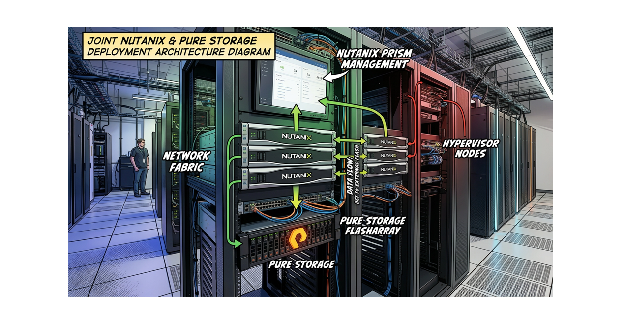
For years, Nutanix was almost synonymous with HCI, where compute and storage live together in the same nodes. That model works exceptionally well for general-purpose workloads, but it has always had a ceiling: when you need more storage capacity or performance, you also have to buy more compute, whether you need it or not.

The formal partnership between Nutanix and Pure Storage, announced at .NEXT 2025 in May, changes that equation. Nutanix AHV can now run as a compute only platform backed by Pure Storage FlashArray over NVMe/TCP. Each Nutanix AOS vDisk maps directly to a FlashArray volume, which means per VM granularity for snapshots, quality-of-service controls, and replication. You get the operational simplicity of Prism as a unified management plane while the FlashArray handles the storage heavy lifting underneath.

This post walks through what it actually takes to build that environment, based on the Cisco FlashStack with Nutanix Installation Field Guide (v1.0, December 2025) and supplemental information from Nutanix and Pure Storage documentation.

Architecture Overview

The deployment model covered here uses Cisco UCS servers (X-series, C-series, or B-series) as compute only nodes, managed by Cisco Intersight in Intersight Managed Mode (IMM). The nodes connect to Cisco UCS Fabric Interconnects (FIs), and those FIs connect upstream to top of rack switches. The Pure Storage FlashArray sits off to the side as a dedicated external storage array, connected to those same ToR switches over NVMe/TCP.

No local storage is used for AOS datastores. The nodes are diskless or have local drives used only for the hypervisor boot.
Storage traffic travels over dedicated VLANs and dedicated vNIC pairs, separate from management and guest VM traffic.
The Nutanix Controller VM (CVM) on each node handles the NVMe/TCP initiator connections to the FlashArray automatically. Administrators do not need to manually configure NVMe initiators.
Prism Central (or Prism Element) is the primary management interface for the cluster, while Cisco Intersight manages the UCS hardware layer.

Software Version Requirements

Before any hardware gets racked, confirm that all components meet the minimum software versions. Using mismatched versions is one of the most common causes of failed deployments.

Component	Minimum Version	Notes
Nutanix AOS	7.5 or later
Nutanix AHV	11.0 or later
Foundation Central	1.10 only	Do not use 2.x at this time
Prism Central	7.5 or later	Required for Licensing
Nutanix LCM	3.3	Included with AOS 7.5
Pure Storage Purity/FA	6.10.3 or later	Upgrade must be done before installation begins
Cisco Fabric Interconnect	4.3(4.240066) or later
Cisco Intersight Virtual Appliance	1.1.5-1 or later	Older CVA/PVA versions will cause failures
Cisco UCS X210c-M7 Firmware	5.4(0.250048) or later
Cisco UCS C-series M6/M7 Firmware	4.3(6.250053) or later
Cisco UCS B-series M5/M6 Firmware	5.3(0.250021) or later

Important: Only Foundation Central version 1.10 should be used. The Appliance VM version 2.x is explicitly not supported for this deployment type. Do not use it.

IP Address Planning

IP address planning should be completed before any configuration begins. Retrofitting addressing after the fact wastes time and introduces risk.

Infrastructure

2 addresses for the Fabric Interconnects
1 address for the Foundation Central Appliance VM
1 optional address for Prism Central / Foundation Central VM

Per Nutanix Host (five addresses each)

AHV hypervisor management address
Controller VM (CVM) management address
CIMC management address (assigned as a pool in Intersight)
Storage interface address, VLAN 1 (assigned as a pool in Prism Element)
Storage interface address, VLAN 2 (assigned as a pool in Prism Element)

Pure Storage FlashArray (seven addresses)

1 per controller management interface
1 roaming array management address
1 per NVMe/TCP storage interface (minimum 4 across two controllers and two VLANs)

Storage addresses must be Layer 2 adjacent to the hosts and cannot traverse a router. Use two separate storage VLANs, one for the A side controller interfaces and one for the B side.

Step 1: Pure Storage FlashArray Configuration

The FlashArray setup is best done via CLI. Some configuration tasks cannot be completed through the Purity GUI. This assumes the array is already racked, cabled, powered on, and reachable on its management network, with Purity/FA 6.10.3 or later already running.

Enable and Configure NVMe/TCP Interfaces

Four Ethernet interfaces need to be assigned to NVMe/TCP. The example below uses interfaces eth10 and eth11 on each controller.

			
# Enable the four storage interfaces
purenetwork eth enable ct0.eth10
purenetwork eth enable ct0.eth11
purenetwork eth enable ct1.eth10
purenetwork eth enable ct1.eth11
# Assign addresses, MTU 9000, and NVMe/TCP service
purenetwork eth setattr --address 10.1.61.100/24 --mtu 9000 --servicelist nvme-tcp ct0.eth10
purenetwork eth setattr --address 10.1.62.100/24 --mtu 9000 --servicelist nvme-tcp ct0.eth11
purenetwork eth setattr --address 10.1.61.101/24 --mtu 9000 --servicelist nvme-tcp ct1.eth10
purenetwork eth setattr --address 10.1.62.101/24 --mtu 9000 --servicelist nvme-tcp ct1.eth11

		

Use MTU 9000 (jumbo frames) wherever possible. If jumbo frames are not supported end to end in your network, set MTU to 1500 and ensure consistency across all components.

Create the Realm, Pod, and Administrative User

			
# Create the Realm for RBAC segmentation
purerealm create <realm_name>
# Create a Pod within the Realm for this Nutanix cluster
purepod create <realm_name>::<pod_name>
# Create the management access policy granting admin rights to the Realm
purepolicy management-access create --role admin --realm <realm_name> <policy_name>
# Create the user Nutanix will use to authenticate to the array
pureadmin create <username> --access-policy <policy_name>

		

Important: Do not use the quota setting on the Pod. Quota is not the correct mechanism here and will not give Nutanix an accurate picture of available storage. Instead, configure Advertised Size on the Pod. Advertised Size tells the FlashArray how much capacity to present to Nutanix regardless of physical consumption, which is what Prism needs to display meaningful storage availability. Set it to a value that reflects the usable capacity you intend to make available to the cluster.

Step 2: Cisco UCS and Intersight Configuration

Configure Fabric Interconnect A first via serial console or HTTPS Express Setup, setting the management mode to Intersight. After FI-A shows a login prompt, configure FI-B. FI-B will detect the peer and prompt to join the cluster.

Once the FIs are up, log into Cisco Intersight and claim the UCS domain using the Device ID and Claim Code from the FI web console. Create Resource Groups and an Organization, create and deploy a Domain Profile to the Fabric Interconnects, and set the System QoS Best Effort MTU to 9216 to allow jumbo frames.

This is where compute only Nutanix deployments require careful attention. Each server needs at least two vNIC pairs: an infrastructure pair for AHV and CVM management traffic, and a dedicated storage pair carrying the NVMe/TCP storage VLANs.

Infrastructure vNIC naming is case sensitive. Foundation Central will reject the deployment if these names are wrong. For a single VIC server use ntnx-infra-1-A on Slot MLOM, PCIe Order 0, Fabric A, Failover disabled and ntnx-infra-1-B on Slot MLOM, PCIe Order 1, Fabric B, Failover disabled.

The LAN Connectivity Policy and the Ethernet Network Group Policy are not shared resources across clusters. Each Nutanix cluster deployment requires its own dedicated LAN Connectivity Policy and its own Ethernet Network Group Policy. This means the full policy set must be created from scratch for every cluster you deploy onto the same UCS domain. Reusing policies across clusters will cause MAC address pool conflicts and VLAN assignment collisions that are difficult to diagnose after the fact. Name them to reflect the cluster they belong to and treat them as cluster-scoped objects from the start.

Step 3: Foundation Central Deployment

For first-time cluster deployments with no existing Nutanix infrastructure, the Appliance VM is the simplest path. Deploy it with 2 vCPUs and 4 GB RAM with a static IP address. DHCP is not supported. Run the setup script from the local console after booting and access the GUI at https://<FC_IP>:9440.

Upload the AOS installation package, its metadata JSON file, and the AHV ISO via API calls to the Appliance VM. Retrieve the hosted file URLs by browsing to http://<FC_IP>:8053/files/images and enter those URLs into the cluster deployment wizard.

Step 4: Nutanix Cluster Deployment

Connect Foundation Central to Cisco Intersight by entering the API Key ID and Secret Key under Settings. The API key user must have at minimum Server Administrator privileges in the relevant Intersight Organization.

Onboard the Cisco UCS servers by selecting Intersight Managed Mode and choosing the target nodes
Select the onboarded nodes and click Create Cluster
Select Compute Cluster (not HCI Cluster, since there is no local storage)
Configure the infrastructure vNIC pair and at least one dedicated storage vNIC pair
Assign IP addresses and hostnames. Use Bulk Configuration to set sequential addresses efficiently
Enter the download URLs for AOS, the AOS metadata file, and the AHV ISO
Set NTP servers, DNS servers, and timezone
Select the Foundation Central API Key and click Create Deployment

Deployments without firmware changes typically complete in 75 to 90 minutes. If firmware upgrades are required, add 60 to 90 minutes.

Step 5: External Storage Connectivity

After the Nutanix cluster is up and accessible in Prism Element, select I’ll Do This Later when prompted to set up external storage. The virtual switch configuration must be done first.

Edit the default virtual switch vs0 to remove any storage vNICs, leaving only the infrastructure vNIC pairs as uplinks
Create a new dedicated storage virtual switch, assign it the storage vNIC pair, set MTU to 9000, and Bond Type to Active-Active with MAC pinning
Create one External Storage Interface per storage VLAN, associated with the new storage virtual switch, with an IP pool large enough for one address per node plus room for growth. Enable the External Storage option and set MTU to 9000.

Before attaching the array, verify jumbo frame connectivity from the CVMs to all four FlashArray storage interfaces:

			
ping -M do -s 8972 10.1.61.100
ping -M do -s 8972 10.1.62.100
ping -M do -s 8972 10.1.61.101
ping -M do -s 8972 10.1.62.101

All four tests should complete with 0% packet loss. From Prism Element, click Attach External Storage, select Pure Storage FlashArray, enter the clustered management IP, the Realm administrative username and password, select the Realm and Pod, and click Attach. The connection typically completes within 30 to 60 seconds.

Step 6: Post-Installation Tasks

Change the default passwords on three accounts on AHV (root, admin, and nutanix) and on the CVM nutanix account. Run the NCC password health check after: ncc health_checks system_checks default_password_check

Run a full NCC health check from Prism Element and resolve all failures and warnings before the cluster goes into production. LCM 3.3 ships with AOS 7.5. Run an inventory job to see available Nutanix software updates. Note that LCM will not perform server firmware updates for compute only nodes connected to external storage.

Remove the Default Pure Storage Protection Policy from Volumes. When the Nutanix cluster attaches the FlashArray and begins using volumes, the array automatically applies a default protection policy to each volume. This is standard Pure Storage behavior, but it is incompatible with Nutanix AOS. Nutanix manages its own data protection and snapshot schedules internally, and the FlashArray protection policy generates snapshots on its own schedule with no coordination with AOS. Those uncoordinated snapshots can cause data consistency issues and will generate NCC warnings. Remove the protection policy from all volumes through the Purity GUI or CLI as soon as the external storage connection is established and before production workloads begin. The volumes continue to function normally without it; Nutanix handles protection from its own layer.

Things Worth Calling Out

vNIC naming. The ntnx-infra-1-A and ntnx-infra-1-B names in the LAN Connectivity Policy are case sensitive. A single capitalization error will cause the deployment to fail at validation. Fix it in the Intersight policy and resubmit.

Foundation Central version. Version 1.10 only. The Appliance VM version 2.x exists and is available, but it does not work with Cisco UCS hardware in this context. Do not use it.

Jumbo frames. The MTU 9000 setting at the vNIC level and the virtual switch level only permits jumbo frames to pass; it does not enforce them. All switching infrastructure between the hosts and the FlashArray interfaces must also support 9000 byte frames. Use the ping test above to verify before attaching the array.

Storage VLAN design. Use two separate storage VLANs, one for the A side controller interfaces and one for the B side. Storage addresses within each VLAN must be in the same Layer 2 domain as the hosts and cannot be routed.

Advertise Size, not quota. Do not use the quota setting on the Pure Storage Pod. Use Advertise Size instead. Quota does not give Nutanix an accurate view of available storage capacity. Advertise Size is the correct mechanism and must be configured before the cluster starts writing data.

Per cluster LAN Connectivity Policy and Ethernet Network Group. These are not shared objects. Every Nutanix cluster on the same UCS domain needs its own dedicated LAN Connectivity Policy and Ethernet Network Group Policy. Sharing them causes MAC address pool conflicts and VLAN assignment collisions that are difficult to diagnose after the fact.

Default Pure Storage protection policy on volumes. The FlashArray automatically attaches a default protection policy to each volume when the cluster connects. Nutanix does not support those uncoordinated snapshots; they conflict with AOS-managed data protection and will trigger NCC warnings. Remove the protection policy from all volumes through Purity before production workloads begin.

Summary

The Nutanix AHV compute only model backed by Pure Storage FlashArray over NVMe/TCP represents a meaningful shift in how converged infrastructure is deployed. It separates the scaling concerns for compute and storage, delivers per VM storage granularity at the array level, and maintains a single management plane through Prism for day to day operations.

The installation process involves more moving parts than a traditional HCI cluster. Cisco Intersight, Foundation Central, Purity CLI, and Prism Element all play distinct roles, and the sequencing matters. Following the steps in order and confirming each layer before moving to the next is the most reliable path to a successful deployment.

For questions about this architecture or assistance planning a deployment, reach out at javier.rodriguez@eplus.com.

Migrating Virtualized Workloads to Nutanix AHV: A Phased Approach That Works in Production

June 3, 2026

Every VMware to Nutanix AHV migration project comes with the same fundamental tension: you want to move workloads to a better platform without disrupting the people who depend on those workloads every day. The good news is that Nutanix Move, when paired with a well defined phased methodology, handles that tension well. This post walks through how we approach these engagements at ePlus, covering the migration mechanics, database specific considerations, and the operational steps that close out each phase cleanly.

How Nutanix Move Works

Nutanix Move is a cross hypervisor mobility tool that automates VM migrations from VMware ESXi, Hyper-V, or public cloud sources to Nutanix AHV. The core model is straightforward: Seed, Sync, Cutover.

Discovery: Connect Move to the source environment (vCenter, standalone ESXi, or Hyper-V) and the target Nutanix cluster. Move inventories the VMs and validates compatibility before anything touches production data.
Data Seeding: Move creates a placeholder VM on the AHV side and begins copying virtual disks from the source. This initial seed runs in the background while the source VM stays live.
Changed Block Tracking (CBT): After the initial copy, Move uses CBT to replicate only blocks that have changed since the last sync. This keeps the replication delta small and the eventual cutover window short.

Why Daytime Replication Is Safe

A common concern when planning migrations is whether running replication during business hours will hurt production performance. In practice, it does not, and here is why.

Non Disruptive Snapshots Move uses native snapshot mechanisms (VMware CBT, for example) to read source data. The VM stays powered on and users experience no interruption.	Network Throttling Move supports bandwidth throttling on migration traffic so replication does not compete with production traffic on shared links during peak hours.
Background Operation The seeding phase is a background task. End users are fully isolated from the process because their application is still running on the source hypervisor.	Incremental Efficiency After the initial seed, subsequent syncs only move changed blocks, so the bandwidth consumption of ongoing replication is a fraction of the initial transfer.

The Cutover Process

The cutover is the only step that involves any downtime, and even that window is typically measured in minutes per VM. The sequence is deterministic and should be documented in the project plan before any work begins.

Final Sync: Move performs one last incremental sync to capture the most recent changed blocks.
Graceful Shutdown: The source VM is powered off cleanly, not forcefully terminated.
Final Delta: A final incremental pass captures any blocks written during the shutdown sequence.
Activation: Move installs the required VirtIO drivers for AHV, optionally reconfigures IP addressing, and powers the VM on within the Nutanix cluster.

Practical Note
For most general purpose VMs, the combined downtime from final sync through power on on AHV is under five minutes. Database VMs with large in flight transactions may take slightly longer depending on the final delta size.

Rollback Strategy

One of the most important things to communicate to stakeholders before a cutover is that rollback is not a complex recovery procedure. It is simply reversing a power state.

Because Move does not delete or modify the source VM during cutover (it only powers it off and disconnects its network interface), the path back to the original state requires no data restoration. If a migrated VM does not perform as expected on AHV, the steps are:

Power off the VM on the Nutanix AHV side.
Reconnect the network interface on the source VM.
Power on the source VM in the original environment.

The source disks remain completely untouched throughout the process, so this rollback takes seconds rather than hours. It also means stakeholder sign off on a cutover carries much lower risk than it would in a traditional migration approach.

Special Migration Scenarios

Not every VM is a candidate for a straightforward Move migration. A few categories require a different approach:

Legacy Operating Systems: Windows Server 2003 and older Linux kernels with unsupported kernel versions are explicitly unsupported by modern versions of Nutanix Move and the standard AHV VirtIO driver set. These workloads cannot use the standard Move migration path and require an alternative approach such as a cold clone, a bare metal backup restoration, or an application level migration to a newly provisioned VM.
Physical Hardware Pass through: VMs with PCI pass through devices or Raw Device Mappings (RDMs) require manual reconfiguration on the target side.
Shared Disk Clustering: Certain older Oracle RAC or MSCS configurations that rely on shared SCSI bus emulation need architectural review before migration.

For these cases, the alternatives range from a manual cold clone, to an application level migration, to a fresh OS installation with data restoration from backup. The right path depends on the workload, and that decision should be made during technical discovery before the project schedule is finalized.

Database Migration Methodology

Databases deserve a separate treatment because the consequences of a failed migration, or even a migration that succeeds but lands on a poorly configured target, are higher than for stateless application servers. We cover both Microsoft SQL Server and Oracle here.

Storage Architecture for Database VMs

Nutanix gives database workloads two primary storage paths: native vDisks and Nutanix Volume Groups.

Native vDisks are the default for AHV VMs and are simple to manage through Prism. Starting with AOS 6.x, the Autonomous Extent Store (AES) improved local sharding for native vDisks, so they are no longer as constrained as they were in earlier releases. That said, a single CVM still serves as the primary I/O path for a given vDisk, which means very high throughput workloads can reach a performance ceiling at the CVM level.
Nutanix Volume Groups (VG) are collections of vDisks presented as block devices. For AHV, VGs can be direct attached, appearing as native SCSI devices to the guest OS. When Volume Group Load Balancing (VGLB) is enabled, the system shards vDisks across all CVMs, removing the single CVM I/O path and allowing the database to draw on the aggregate throughput of the entire cluster’s Stargate processes.

iSER Support: For the highest performance requirements, Nutanix supports iSER (iSCSI Extensions for RDMA), which bypasses the TCP/IP stack entirely to reduce latency and CPU overhead between the guest and the CVM. This is worth evaluating for latency sensitive OLTP workloads.

AHV Specific Tuning for Databases

Several AHV configuration decisions have a direct and measurable impact on database performance.

vCPU to pCPU Ratio: For production databases, size assuming 1 vCPU equals 1 physical core, not one hyperthreaded thread. Oversubscription introduces CPU Ready Time, which is particularly harmful to latency sensitive query workloads. Target below 5% CPU Ready.
Memory Reservations: Reserve 100% of assigned VM memory for SQL Server and Oracle VMs. AHV memory reclamation through ballooning or swapping can cause significant and hard to diagnose latency spikes in database workloads.
Huge Pages: AHV uses 2 MB Huge Pages to reduce Translation Lookaside Buffer (TLB) pressure. Ensure the guest OS is configured to use large page allocations to take advantage of this.
vNUMA: For VMs larger than a single physical socket, enable vNUMA and match the virtual topology to the physical hardware. This allows the database engine to schedule threads and memory access with NUMA awareness. Disable CPU hot add, as enabling it disables vNUMA and can cause performance degradation of up to 30%.

AOS Features That Matter for Databases

Data Locality AOS stores a VM’s data on the same physical node where the VM runs. Read I/O is served locally without network traversal, which reduces database read latency materially.	AHV Turbo (Frodo I/O Path) Bypasses traditional QEMU emulation with a multi-queue I/O path that scales with the number of vCPUs, delivering higher I/O capacity and lower CPU overhead for storage intensive workloads.
Nutanix Blockstore A block management system that moves device interactions into user space, eliminating context switching and kernel driver overhead for data disks.	VGLB for OLAP Volume Group Load Balancing distributes I/O across all CVMs in the cluster. Critical for high throughput OLAP and reporting workloads that can saturate a single CVM.

Microsoft SQL Server Migration Options

There are three viable paths for SQL Server migrations, and the right choice depends on the deployment type and the acceptable downtime window.

Nutanix Move: The simplest path for standalone instances. Move handles disk conversion to AHV RAW format, VirtIO driver injection, and IP configuration. Best suited for standalone instances where a brief cutover window is acceptable.
Always On Availability Groups: Build a new SQL VM on AHV, join it to the existing Windows Server Failover Cluster (WSFC), and add it as a new secondary AG replica. Once synchronized, perform a planned manual failover to promote the Nutanix based node, then decommission the old nodes. This approach reduces cutover risk for business critical SQL workloads and can achieve near zero application downtime.
Backup and Restore: Take a full backup of the source database, restore it on a pre staged SQL VM on AHV using WITH NORECOVERY, and during the cutover window take a tail log backup, restore it with WITH RECOVERY, and redirect applications to the new instance.

Oracle Migration Options

Nutanix Move: Recommended for migrating the Oracle VM as is from vSphere to AHV when the VM itself is in Move’s compatibility matrix. Move handles VirtIO driver injection automatically.
RMAN Active Duplication: Use Oracle Recovery Manager to perform an active duplication from the source to a new Oracle VM on AHV. The source database remains online until the final switchover, minimizing the downtime window.
Data Guard: Set up a physical standby on the Nutanix cluster, synchronize it via RMAN, and then perform a Data Guard switchover to promote the Nutanix instance to primary. This is the lowest risk option for Oracle databases with strict RPO/RTO requirements.
Oracle RAC with Nutanix Volumes: For RAC deployments, Nutanix Volumes provide the shared block storage required by clusterware. Volume Groups should be attached via iSCSI and configured with SCSI-3 Persistent Reservations.

SQL Server Best Practices on AHV

These configurations should be treated as baseline for any production SQL Server on Nutanix, whether migrated or newly deployed.

Storage Layout

Use at least four vDisks to distribute data files, log files, TempDB, and the OS independently.
Format all data and log volumes with a 64 KB NTFS allocation unit size.
Do not use Windows Dynamic Disks or in guest volume managers. Add vDisks directly to the VM instead.
Keep OS, SQL binaries, user database data, logs, and TempDB on separate volumes.

Instance Level Tuning

Instant File Initialization (IFI): Grant the SQL Server service account the “Perform Volume Maintenance Tasks” privilege to enable IFI. This eliminates zero initialization overhead during data file creation and auto growth events. IFI applies only to data files (.mdf and .ndf). Log files (.ldf) are always zero initialized regardless of this setting. Starting with SQL Server 2016, IFI can also be enabled directly from the installation wizard.
Lock Pages in Memory (LPIM): Enable LPIM to prevent Windows from paging the SQL Server buffer pool to disk. Max Server Memory must be set correctly before enabling LPIM to avoid starving the guest OS.
Max Server Memory: For mid to large VMs, leave 6 to 8 GB for the OS. For VMs under 32 GB of RAM, 4 GB is often sufficient. A practical formula: reserve 10% of total RAM for the OS, with a ceiling of around 8 GB unless SSIS or SSRS also run on the same instance.
MAXDOP: Set MAXDOP to the number of logical cores within a single vNUMA node. For SQL Server 2016 and later, the updated guidance is to use either 8 or the number of cores per NUMA node, whichever is smaller.
Cost Threshold for Parallelism (CTFP): Increase from the default of 5 to at least 50. OLTP workloads land at 50. Hybrid environments sometimes use a value in the 25 to 50 range.
TempDB: Match the number of data files to the logical processor count when that count is 8 or fewer. Start at 8 data files when the logical processor count exceeds 8. Only increase beyond 8 (in increments of 4) if PAGELATCH_UP or PAGELATCH_SH waits confirm actual contention.

SQL Server Baseline Configuration Summary

Setting	Recommended Baseline	Reason
IFI	Enabled	Eliminates zero initialization overhead for data files during creation and auto growth.
LPIM	Enabled	Prevents Windows from reclaiming the SQL Server buffer pool. Requires Max Server Memory to be set first.
Max Server Memory	Total RAM minus 4 to 8 GB (or 10% of total RAM)	Prevents SQL Server from starving the guest OS.
MAXDOP	8 or cores per NUMA node, whichever is smaller	Keeps parallel query execution within a single NUMA domain.
CTFP	50 (or 25 to 50 for hybrid workloads)	Prevents low cost queries from triggering parallelism on modern multi core hardware.
TempDB	Match logical processor count up to 8; increase by 4 only when contention is confirmed	Reduces allocation contention. All files must be equally sized with identical growth settings.

Oracle Best Practices on AHV

Oracle on Nutanix AHV benefits from the same platform level advantages as any other workload, but the database engine has enough specific tuning requirements that it warrants its own treatment.

Memory Allocation: SGA and PGA

Reserve approximately 10 percent of the total VM memory for the guest OS and file cache. Of the remaining 90 percent, allocate 80 percent to the System Global Area (SGA) and the remaining 20 percent to the Program Global Area (PGA). Memory reservations should be set to 100% of the assigned VM memory. Memory overcommit is not recommended for Oracle workloads.

Storage Layout and Disk Groups

NDB provisions multiple vDisks spread across ASM disk groups to maximize throughput across the Distributed Storage Fabric. The two primary disk groups are DATADG for database data files and RECODG for redo logs and archive files. For Oracle RAC, a third disk group CRSDG is required for Grid Infrastructure and clusterware files.

Disk Group	Small or Medium (500 GB and under)	Large (501 GB and above)
CRSDG (RAC only)	3 vDisks	3 vDisks
DATADG	4 vDisks	8 vDisks
RECODG	2 vDisks	4 vDisks

ASM Configuration Options

Nutanix supports ASMFD (ASM Filter Driver), ASMLIB, and udev rules for ASM disk mappings. ASMFD is the preferred method on modern Linux distributions. All ASM disks should be placed on vDisks in an AOS storage container with inline compression enabled and deduplication disabled.

Network Design for Oracle RAC

Oracle RAC requires a public network for client connections and a private interconnect for cache fusion on separate VLANs. Mixing them on the same VLAN introduces the risk of cache fusion traffic competing with client traffic. When using NDB to provision Oracle RAC, NDB manages IP address assignment across public, private, and virtual (scan and VIP) network types.

RAC and Nutanix Volumes: Oracle RAC requires shared storage for the CRSDG disk group. On AHV, this is provided through Nutanix Volume Groups attached via iSCSI with SCSI-3 Persistent Reservations enabled. This is a prerequisite for RAC clusterware to function correctly.

Oracle Patching with NDB

NDB uses an out of place patching model for Oracle. Rather than patching a running Oracle home directly, the process involves provisioning a new database VM from an existing software profile, manually applying the patch set to that VM, and then creating a new software profile version from the patched VM. Once published, that version becomes available to all Oracle VMs managed by NDB. Patching can be performed in either a rolling or non rolling fashion for Oracle RAC environments.

Time Machine Backup and Recovery for Oracle

NDB Time Machine creates application consistent snapshots of Oracle databases along with copies of transaction log files. An SLA attached to the time machine controls snapshot frequency and retention. Point in time recovery is available as long as both a base snapshot and the covering transaction logs exist for the target timestamp. NDB restores the vDisks from the appropriate snapshot and then applies log files forward to bring the database to a consistent state.

Decommissioning Protocol

The migration is not complete when the VM powers on successfully on AHV. A structured decommissioning process ensures the legacy environment is cleaned up safely.

Step	Action	Owner
1	Source VMs remain powered off with NIC disconnected for a 48 to 72 hour burn in period to prevent IP conflicts.	Infrastructure Team
2	Confirm with Application Owners that performance and stability on AHV is acceptable after the burn in period.	Project Lead
3	Archive a final backup of the source VM according to the organization’s retention policy before deletion.	Backup Admin
4	Remove the VM from the source cluster inventory.	Infrastructure Team
5	Update the CMDB or asset tracker to reflect the VM’s new hypervisor and decommission the legacy record.	IT Operations

Technical Discovery Requirements

The quality of the discovery work done before migration determines how smooth everything else goes. At a minimum, the following information should be gathered before any migration plan is finalized.

General Infrastructure

Specific vSphere version and ESXi build number in use on source hosts
Networking configuration: LACP, Jumbo Frames (MTU 9000), or standard configuration
IP retention requirement: retain existing IPs after migration or assign new IPs on AHV
Guest OS list with versions and BIOS/UEFI boot mode for each VM in scope

SQL Server Environments

SQL Server versions and editions (Standard vs. Enterprise) deployed
Deployment type: Standalone, Failover Cluster Instance (FCI), or Always On AG
Current vCPU to physical core allocation and whether LPIM is already configured
vDisk layout per VM: number of disks, purpose (Data, Log, TempDB), and whether any single large data files exist that should be split
Dependencies on MSDTC, Linked Servers, or SQL Agent Jobs that require documentation before cutover

Oracle Environments

Oracle versions in scope and whether instances are Single Instance or RAC
Shared storage configuration for RAC: ASM with ASMLib, ASMFD, or udev rules
Huge Pages configuration status in the guest OS
Existing RMAN backup workflows or Data Guard standbys that can be leveraged
Source platform architecture: if any workloads currently run on AIX or Solaris (SPARC), be aware that Nutanix Move is strictly an x86-to-x86 tool and cannot be used for these migrations. AIX and Solaris on SPARC are Big-Endian, while Nutanix AHV runs exclusively on x86-64 (Little-Endian). Cross-endian migrations require a fully manual path using RMAN CONVERT for Oracle or an application level export and restore, and should be scoped separately from the rest of the Move migration plan.

Migration Constraints

Maximum acceptable maintenance window for final cutover
Average daily change rate for production databases (drives seeding bandwidth planning)
Top 10 application functions or queries to validate Day 1 performance after migration
Total allocated versus used storage per database environment, plus expected annual growth